Authors: Linstädter A1,2, Töpper JP3,4
Reviewer: Tielbörger K5
Measurement unit: counts and mm; Measurement scale: plot; Equipment costs: €€; Running costs: €; Installation effort: low; Maintenance effort: low; Knowledge need: medium; Measurement mode: manual
Plant demography is the study of population size (abundance) and its underlying parameters. It describes the state of a particular population of a species and how this state changes through time (Gibson, 2015). Following a population and recording demographic variables for consecutive time steps allows us to build population models (Caswell, 2001; Merow et al., 2014a). With these models we can study the mechanisms of abundance changes. Key questions for climate-change studies would be, for example, “Does the population size decline because of an increased mortality or due to a reduced reproduction?” or “Does the population structure change during population decline, i.e. are certain plant sizes, ages, or stages declining more than others?” The processes underlying changes in population size are called “vital rates” (Franco & Silvertown, 2004). These are survival, individual growth, and fecundity (sexual and clonal reproduction). In addition, the classical demographic equation also includes immigration and emigration. Such mechanistic insights improve our understanding of the ecological processes linking changing environmental conditions to abundance responses (Fridley, 2017; Töpper et al., 2018). Climate-change studies providing such links through demographic approaches thus contribute to generating more accurate projections of future vegetation responses (Pagel & Schurr, 2012; Merow et al., 2014b) and lead to more effective measures in mitigation, conservation, and restoration contexts (Elzinga et al., 1998). Studies on plant demography and population modelling are particularly well suited to investigate mechanistic responses of plant populations to a range of environmental and other global-change drivers and changes in these drivers. These can be either observational studies of, for example, climate (Adler & HilleRisLambers, 2008; Dalgleish et al., 2011; Nicole et al., 2011; Sletvold et al., 2013; Shryock et al., 2014; Treurnicht et al., 2016), competition/facilitation (Buckley et al., 2003; Adler & HilleRisLambers, 2008), fire frequency (Evans et al., 2010), land use (van der Meer et al., 2014; Johansen et al., 2016), herbivory (Miller et al., 2009), and nitrogen deposition (Nicole et al. 2011), or experimental studies of climate (Pfeifer-Meister et al., 2013; Salguero-Gomez et al., 2013; Farrer et al., 2014; Gornish, 2014; Töpper et al., 2018; Cui et al. 2018), competition/facilitation (Olsen et al., 2016), land use (Ehrlén et al., 2005; Sletvold et al., 2013), and nitrogen deposition (Farrer et al. 2014, Gornish 2014).
4.3.1 What and how to measure?
Sampling strategy
The two cardinal aspects of plant demography (abundance and vital rates) require specific consideration when designing the sampling strategy for a climate-change study. As most studies are set up in small-stature vegetation such as grasslands, the following sections mainly refer to herbaceous and small woody plant species; see section 4.3.2 for specific recommendations for trees and large shrubs. A complete census of a plant population is rarely feasible (Gibson, 2015); hence population size and its temporal variation is usually estimated in study plots (Gross, 2002, but see Münzbergová & Ehrlén, 2005 for alternatives). The minimum number of individuals required to build population models ranges from 300–400 for matrix projection models and down to c. 100 for regression-based integral projection models (cf. Ramula et al., 2009). Note that lower numbers may also work for rare and/or endangered species for example, under the regression approach, as long as the individual regressions can be parameterised appropriately. Usually these numbers cannot be accommodated in a single study plot, and hence, the adequate number, size, and minimum distance of study plots needs to be determined depending on the size and average density of the study species. Large and rare plants require larger plots (or more plots if the study approach restricts plot size to a certain limit); the guidelines for the minimum size of plots for aboveground biomass estimation (see protocol 2.1.1 Aboveground plant biomass) may be used as a rough guideline for the maximum size of demographic study plots within the framework of climate-change studies. As with aboveground biomass plots, we recommend a nested plot design (Figure 2.1.1.1a in protocol 2.1.1 Aboveground plant biomass) or a multi-plot approach (Figure 2.1.1.1b in the same protocol).
For herbaceous vegetation, plot size ranges from 4 m² for the savanna bunchgrass Stipagrostis uniplumis (Zimmermann et al., 2008), over 1 m2 for the perennial forb Plantago lanceolata (Wardle et al., 2014), 0.0625 m2 for the small perennial forb Viola biflora (Olsen et al., 2016; Töpper et al., 2018), and down to 0.04 m2 and 0.01 m² for the small annual forbs Carrichtera annua (Salguero-Gomez et al., 2012) and Arabidopsis thaliana, respectively (see Figure 4.3.1C). Plots are usually randomly chosen, but with the obvious restriction that they need to contain the study species (unless “empty” plots are of particular purpose, e.g. when studying invasiveness). Unless one is already very familiar with the plant species’ morphology and phenology, as well as with other organisms in the habitat (such as herbivores), it is highly recommended to carry out a pilot study for testing the efficiency of field methods and for an assessment of the study design (Gibson, 2015).
When installing the study plots it is important to mark them properly so that plot position is stable and easy to retrieve. A good approach is to mark plot corners (see protocol 2.1.1 Aboveground plant biomass for details). Aboveground plot tags and individual tags should be replaced immediately when discovered to be damaged or removed (e.g. through animal trampling, snow movement, or human interference). When studying species that can “move” by means of vegetative growth, it is important to deal with emigrants and immigrants properly so as to ensure no bias is introduced. Migration can be studied as yet another “vital rate”, but it can also be excluded if not relevant to the research question.
Estimating abundance
Gold standard
For plant abundance, individuals of the study population are counted in each study plot.
Bronze standard
Counting can be challenging for clonal plants; here usually proxies such as cover or presence in sub-plots are used and they serve as relative measures of abundance (e.g. for comparing climate-manipulation treatments, see also protocol 2.1.1 Aboveground plant biomass).
Measuring vital rates
The vital rates of survival, growth, and fecundity are highly variable in time and require repeated observations of plant populations in the field. They can be assessed from the same study plots used for abundance estimation by linking the state of the population in sampling event t+1 to that of the previous sampling event t. Please note that other variables such as seed viability and germinability also contribute to plant demography. However, these variables do not require a repeated observation of plant populations in the field; see protocol 4.2 Seed viability, germinability and dormancy for their respective sampling protocols.
Measuring survival
Gold standard
The gold standard for measuring survival requires marking individuals and monitoring their fate over time. Survival is then measured by re-finding a living individual recorded at the previous sampling event. For very dense populations, monitoring all individuals within the study plots might be too time-consuming, and a subsample of individuals may be monitored per plot. Note that the total population size in all replicate plots of a population (i.e. experimental treatment, gradient level) should still reach the recommended minimum number of individuals (see above).
Keeping track of each individual plant’s identity is critical (Gibson, 2015). This can either be ensured by tags or marks placed next to the individual plant (options 1–5 in Table 4.3.1), or by tagging or marking the individuals themselves (options 6–12 in Table 4.3.1, where we also give the main advantages and disadvantages of the alternative methods). Practical details can be derived from an illustration of recommended options (Figure 4.3.1). Another option that could also be combined with physical marks is to record individual plants using repeat photography. This approach is particularly valuable for plants with a well-defined canopy, such as perennial bunchgrasses (Zimmermann et al., 2015). It could also be used for tree populations, where aerial photography is preferable. In general, it is advisable to note each individual’s position by measuring co-ordinates within the study plots (Gibson, 2015). This information can be used to create population maps for the study plots: another useful way for monitoring individuals.
Bronze standard
The bronze standard for survival is performing a census of the established study plots during repeated sampling events: a survival rate is then calculated per plot. This census approach is easier and less time-consuming than monitoring individuals’ fates: however it does not allow the monitoring of individual performance.
Measuring growth
Gold standard
Growth is estimated as the change in “developmental state” of surviving individuals from one sampling event to the next. The developmental state is described by a state variable, such as measures of stage, age, or size, which depends on the species’ life-form and cycle. As plant species often lack the well-defined stages found in animals (but see Jongejans & de Kroon, 2005) and age is hard to assess, tracking an individual plant’s size is the gold standard for estimating growth. For herbaceous species and small woody species (e.g. bilberry – Vaccinium myrtillus), plant size can be estimated via a direct measure of a single trait such as plant height, or the tuft area of bunchgrasses (Zimmermann et al., 2015), or rosette area (Jongejans et al., 2011). However, plant size can also be estimated as aboveground biomass (dry mass), based on several measured plant traits (Wardle et al., 2014; Seldal et al., 2017).
Bronze standard
Similar to plant abundance, growth can also be assessed more rapidly as average growth per plot. For this purpose, changes in a population’s average plant size or biomass are tracked on observation plots. For monospecific stands, changes in plot-level biomass can be used to estimate a population’s growth rate (see protocol 2.1.1 Aboveground plant biomass for details on measuring aboveground biomass). If plant abundance is known for an observation plot, average individual growth rate per plot and individual can be calculated. Again, the bronze standard does not typically allow tracking of individual performance. In the case of clonal plants though, a plot approach may be the only feasible option.
Measuring fecundity
Gold standard
Fecundity comprises both sexual and clonal reproduction (but note that clonality can also be classified as a separate vital rate; e.g. Töpper et al., 2018). Assessing fecundity thus implies a series of measures that links the outcome of sexual and/or clonal reproduction in year t+1, i.e. number and size of established recruits (seedlings or clones), to the state variable of individuals present in year t. In practice, this usually includes measures of whether or not an individual produces seeds or asexual propagules, the number of propagules produced, and the number and size of recruits. This would require, ideally, monitoring the fate of seeds or asexual propagules through the consecutive stages of the recruitment process, which are emergence, survival, and growth through the growing season and survival through the unfavourable season (Zimmermann et al., 2008). Monitoring the individual fate of sexual and asexual recruits is very time-consuming, hence we recommend more rapid methods as a gold standard. Seedlings should only be counted in study plots. In cases of clonal growth, it might additionally be required to note their position on a plot map to be able to separate them from eventual clonal recruits at the following census. A seedling’s individual fate commences being tracked if they have survived the first unfavourable season (see Wardle et al., 2014; PlantPopNet protocol, nd). Similarly, clonal reproduction is best recorded when finding clonal recruits the following year. Seed production is often measured indirectly via the number of flowers or fruits and a constant describing the number of seeds per fruit. Measurement of plant sexual reproduction is more closely described in protocol 4.1 Sexual plant reproduction.
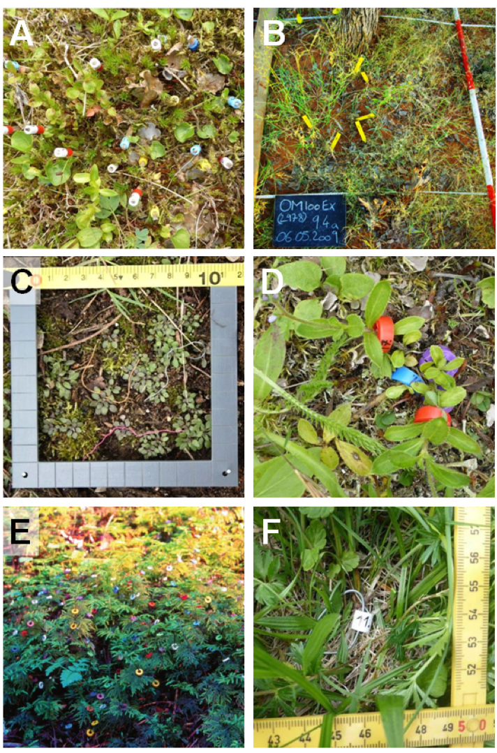
Figure 4.3.1 Recommended tags and marks in plant population biology. A: Wooden toothpicks labelled with numbered and colour-coded beads on top, placed to the left of individuals of Viola biflora (yellow), V. palustris (blue), and Veronica alpina (white and red). B: Labelled plastic stakes placed close to individuals of the perennial bunchgrass Stipagrostis uniplumis monitored in a 1 m² study plot. C: Colour-coded thread loops at the rosette base of Arabidopsis thaliana individuals monitored in a 1 dm² study plot. D: Numbered, colour-coded plastic rings around the basal stems of Veronica officinalis individuals. E: Numbered, colour-coded plastic rings marking clonal segments of the moss Hylocomium splendens. F: Metal wire loops labelled with a numbered plastic bead at the rosette base of Plantago lanceolata individuals; one end of the loop in place. Photo credits: A, D, F: Siri Lie Olsen; B, C: Anja Linstädter; E: Knut Rydgren.
|
Table 4.3.1 Tags and marks used in plant population ecology with their main advantages and disadvantages, and with recommendations for their use. Options 1–5 are placed next to the plant while options 6–12 are placed on the plant. Table modified and extended from Gibson (2015). |
||||||
| Tag or mark | Costs | Effort | Durability | Coding | Disadvantages | Our recommendation |
| 1. Toothpicks | Low | Low | Very low | Numbered beads | Coding difficult; easily lost | For small plants; good for geophytes (Figure 4.3.1A) |
| 2. Wooden stakes | Low | Low | Low | Flags | Will rot, markings will fade | Not recommended |
| 3. Plastic stakes | Medium | Low | Low | Numbers on stakes or flags | Easily lost (lightweight) | For isolated herbaceous plants (Figure 4.3.1B) |
| 4. Metal stake flags | High | Low | Medium | Flags | Plastic flags fade and rip quickly | For isolated herbaceous plants |
| 5. Metal stakes | High | Low to high | Very high | Flags; numbers welded onto stakes | Expensive; may be stolen due to material value | For > 5 year studies on herbaceous plants |
| 6. Thread | Low | Medium | Low | Colour coding | Difficult to create a loop | For small rosette plants (Figure 4.3.1C) |
| 7. Paint or ink marks on leaves | Low | Low | Very low | Colour coding | Can fade or wash off; potentially toxic | Not recommended |
| 8. Plastic straw collars | Low | Medium | Low | Flags | Easily lost | Not recommended |
| 9. Plastic rings | Medium | Low | Medium | Numbers; colour coding possible | Not suitable for very small plants | Flexible, durable system for herbaceous plants (Figure 4.3.1D); also for clonal plants (Figure 4.3.1E) |
| 10. Wire loops | Medium | Medium | High | Flags | Time-consuming to install | Durable system; for woody plants (stem), rosette plants (base, with rod, Figure 4.3.1F) |
| 11. Steel or aluminium tags | High | High | Very high | Colour coding; number stamped on tag | Expensive and time-consuming to install | Very durable; for woody plants |
| 12. Paint marks on stem | Low | Low | Medium | Colour or number coding | Can fade or wash off | Easily discernible; for woody plants (in combination with metal tags) |
The link between seeds and seedlings has to be established through germination and seed-bank experiments (if the species maintains a seed bank), yielding the probability of a seed becoming an established seedling at the following census and the probability of ungerminated seeds surviving in the soil (e.g. Quintana-Ascencio et al., 2003; Zimmermann et al., 2008; see also protocols 4.2 Seed viability, germinability, and dormancy and 4.6 The soil seed bank (buried seed pool)). The specific measurements for vital rate estimation vary between species based on their life cycle, the vital rates involved, and the chosen state variable. It is thus crucial to understand the life cycle of the study species prior to doing a demographic study. Another important consideration to be addressed is whether the population is to be measured before or after reproduction (pre-reproduction census v. post-reproduction census), as this has crucial implications for the life-cycle graph that underpins further analysis of the demographic data (Caswell, 2001). Furthermore, the appropriate number of censuses may vary between certain groups of species. While there is usually one census per year for perennial plant species, annuals require several censuses per year (e.g. Salguero-Gomez et al., 2012). For very short-lived annual plants, such as Arabidopsis thaliana, biweekly visits are appropriate (Arany et al., 2005).
Where to start
Gibson (2015), Gross (2002)
4.3.2 Special cases, emerging issues, and challenges
Measuring species that exhibit vegetative dormancy. These species constitute a special case in terms of life cycle and modelling of demographic data (Lesica & Steele, 1994). Individuals might fail to sprout for one or more years before showing up again. In such species, it is impossible to determine in the field whether a missing plant is dormant or dead. Monitoring a population for several years can yield that information, the necessary time-span being dependent on the maximum number of years an individual of the study species can remain dormant. However, at both start and end of the demographic study, there will be some years where it will be impossible to distinguish transitions out of dormancy from clonal recruitment (start) and transitions into dormancy from mortality (end). In long-term studies, the start- and end-years are hence often excluded from analysis (Gremer et al., 2012), or unobservable life-states can be statistically modelled (Shefferson et al., 2001). In short-term studies, usually neither of these approaches are possible and researchers are hence forced to make assumptions about whether an unobserved plant is dead or dormant (Olsen et al., 2016; Töpper et al., 2018).
Measuring trees and larges shrubs. Given the temporal and spatial scale of climate-change studies, full demographic studies are often not feasible for these long-lived woody species. In the add-on protocol to the International Drought Experiment for tall stature ecosystems (IDE, 2016), it is recommended to only monitor the dieback and survival of adult trees. However, if a climate-change study is specifically set up in vegetation dominated by trees and large shrubs, the gold standard would be to additionally measure i) growth and ii) fecundity, i.e. the germination and fate of tree seedlings and saplings. Specific options for tagging large woody plants are given in Table 4.3.1. Numerous allometric models have been established to estimate the size of trees and shrubs (and, hence, growth) based on one or few state variables (see compilation of models by Henry et al., 2013). Among these variables, “stem diameter at breast height” (dbh; measured at 1.3 m above the ground) is the most prominent one. Although growth is most often measured via annual censuses or over longer periods (Malhi et al., 2004), intra-annual measurements are also possible, for example with the aid of dendrometer bands (McMahon & Parker, 2015). For tropical trees, a single allometric model has recently been established that provides reliable estimates of tree size (biomass) based on only three state variables – stem diameter, tree height, and wood specific gravity (Chave et al., 2014). This model allows the estimation of individual-level and stand-level growth (see protocol 2.1.1 Aboveground plant biomass).
Building population models. In addition to simple statistical analysis of demographic variables of interest, a demographic dataset addressing the entire lifecycle of a species can be used to build population models. The major modelling techniques available for this today comprise “matrix models” (Caswell, 2001) for annual and perennial plants and “integral projection models” (Easterling et al., 2000) for perennials. Another upcoming method is “integrated population models”, a Bayesian modelling approach capable of integrating demographic data from different sources such as field trials and museum materials (Kéry & Schaub, 2012).
4.3.3 References
Theory, significance, and large datasets
Caswell (2001), Easterling et al. (2000), Henry et al. (2013), Merow et al. (2014a), Rydgren & Økland (2002), Salguero-Gomez et al. (2015)
More on methods and existing protocols
Gibson (2015), PlantPopNet protocol (nd), Wardle et al. (2014)
All references
Adler, P. B. & HilleRisLambers, J. (2008). The influence of climate and species composition on the population dynamics of ten prairie forbs. Ecology, 89(11), 3049-3060.
Arany, A. M., de Jong, T., & van der Meijden, E. (2005). Herbivory and abiotic factors affect population dynamics of Arabidopsis thaliana in a sand dune area. Plant Biology, 7, 549-556.
Buckley, Y. M., Briese, D. T., & Rees, M. (2003). Demography and management of the invasive plant species Hypericum perforatum. II. Construction and use of an individual-based model to predict population dynamics and the effects of management strategies. Journal of Applied Ecology, 40(3), 494-507.
Caswell, H. (2001). Matrix Population Models: Construction, Analysis, and Interpretation (2nd ed). Sunderland, Massachusetts: Sinauer Associates, Inc. Publishers.
Chave, J., Réjou-Méchain, M., Búrquez, A., Chidumayo, E., Colgan, M. S., Delitti, W. B. C., … Vieilledent, G. (2014). Improved allometric models to estimate the aboveground biomass of tropical trees. Global Change Biology, 20, 3177-3190.
Cui, H., Töpper, J. P., Yang, Y., Vandvik, V., & Wang, G. (2018). Plastic population effects and conservative leaf traits in a reciprocal transplant experiment simulating climate warming in the Himalayas. Frontiers in Plant Science, 9, 1069.
Dalgleish, H. J., Koons, D. N., Hooten, M. B., Moffet, C. A., & Adler, P. B. (2011). Climate influences the demography of three dominant sagebrush steppe plants. Ecology, 92(1), 75-85.
Easterling, M. R., Ellner, S. P., & Dixon, P. M. (2000). Size-specific sensitivity: Applying a new structured population model. Ecology, 81, 694-708.
Ehrlén, J., Syrjänen, K., Leimu, R., Begona Garcia, M., & Lehtilä, K. (2005). Land use and population growth of Primula veris: an experimental demographic approach. Journal of Applied Ecology, 42(2), 317-326.
Elzinga, C. L., Salzer, D. W., & Willoughby, J. W. (1998). Measuring and Monitoring Plant Populations. Denver, USA: Bureau of Land Management, U.S. Department of the Interior.
Evans, M. E. K., Holsinger, K. E., & Menges, E. S. (2010). Fire, vital rates, and population viability: a hierarchical Bayesian analysis of the endangered Florida scrub mint. Ecological Monographs, 80(4), 627-649.
Farrer, E. C., Ashton, I. W., Knape, J., & Suding, K. N. (2014). Separating direct and indirect effects of global change: a population dynamic modeling approach using readily available field data. Global Change Biology, 20(4), 1238-1250.
Franco, M., & Silvertown, J. (2004). A comparative demography of plants based upon elasticities of vital rates. Ecology, 85, 531-538.
Fridley, J. D. (2017). Plant energetics and the synthesis of population and ecosystem ecology. Journal of Ecology, 105, 95-110.
Gibson, D. J. (2015). Methods in Comparative Plant Population Ecology. Oxford: Oxford University Press.
Gornish, E. S. (2014). Demographic effects of warming, elevated soil nitrogen and thinning on the colonization of a perennial plant. Population Ecology, 56(4), 645-656.
Gremer, J. R., Crone, E. E., & Lesica, P. (2012). Are dormant plants hedging their bets? Demographic consequences of prolonged dormancy in variable environments. The American Naturalist, 179, 315-327.
Gross, K. (2002). Efficient data collection for estimating growth rates of structured populations. Ecology, 83, 1762-1767.
Henry, M., Bombelli, A., Trotta, C., Alessandrini, A., Birigazzi, L., Sola, G., … Valentini, R. (2013). GlobAllomeTree: international platform for tree allometric equations to support volume, biomass and carbon assessment. Iforest – Biogeosciences and Forestry, 6, 326.
IDE (2016). Protocol: Drought Experiments in tall stature (forest and shrubland) ecosystems. Add-On protocol to the International Drought Experiment. http://wp.natsci.colostate.edu/droughtnet/files/2016/12/IDE_Forest-Protocol_final_3.2.pdf (accessed Oct 6 2017)
Johansen, L., Wehn, S., & Hovstad, K. A. (2016). Clonal growth buffers the effect of grazing management on the population growth rate of a perennial grassland herb. Flora, 223, 11-18.
Jongejans, E., & de Kroon, H. (2005). Space versus time variation in the population dynamics of three co-occurring perennial herbs. Journal of Ecology, 93, 681-692.
Jongejans, E., Shea, K., Skarpaas, O., Kelly, D., & Ellner, S. P. (2011). Importance of individual and environmental variation for invasive species spread: a spatial integral projection model. Ecology, 92(1), 86-97.
Kéry, M., & Schaub, M. (2012). Bayesian Population Analysis using WinBUGS – A Hierarchical Perspective. Academic Press.
Lesica, P., & Steele, B. M. (1994). Prolonged dormancy in vascular plants and implications for monitoring studies. Natural Areas Journal, 14(3), 209-212.
Malhi, Y., Baker, T. R., Phillips, O. L., Almeida, S., Alvarez, E., Arroyo, L., … Higuchi, N. (2004). The above‐ground coarse wood productivity of 104 Neotropical forest plots. Global Change Biology, 10, 563-591.
McMahon, S. M., & Parker, G. G. (2015). A general model of intra‐annual tree growth using dendrometer bands. Ecology and Evolution, 5, 243-254.
Merow, C., Dahlgren, J. P., Metcalf, C. J. E., Childs, D. Z., Evans, M. E. K., Jongejans, E., … McMahon, S. M. (2014a). Advancing population ecology with integral projection models: a practical guide. Methods in Ecology and Evolution, 5(2), 99-110.
Merow, C., Latimer, A. M., Wilson, A. M., McMahon, S. M., Rebelo, A. G., Silander, J. A. (2014b). On using integral projection models to generate demographically driven predictions of species’ distributions: development and validation using sparse data. Ecography, 37, 1167-1183.
Miller, T. E. X., Louda, S. M., Rose, K. A., & Eckberg, J. O. (2009). Impacts of insect herbivory on cactus population dynamics: experimental demography across an environmental gradient. Ecological Monographs, 79(1), 155-172.
Münzbergová, Z., & Ehrlén, J. (2005). How best to collect demographic data for population viability analysis models. Journal of Applied Ecology, 42, 1115-1120.
Nicolè, F., Dahlgren, J. P., Vivat, A., Till‐Bottraud, I., & Ehrlén, J. (2011). Interdependent effects of habitat quality and climate on population growth of an endangered plant. Journal of Ecology, 99(5), 1211-1218.
Olsen, S. L., Töpper, J. P., Skarpaas, O., Vandvik, V., & Klanderud, K. (2016). From facilitation to competition: temperature-driven shift in dominant plant interactions affects population dynamics in semi-natural grasslands. Global Change Biology, 22, 1915-1926.
Pagel, J., & Schurr, F. M. (2012). Forecasting species ranges by statistical estimation of ecological niches and spatial population dynamics. Global Ecology and Biogeography, 21, 293-304.
Pfeifer-Meister, L., Bridgham, S. D., Little, C. J., Reynolds, L. L., Goklany, M. E., & Johnson, B. R. (2013). Pushing the limit: experimental evidence of climate effects on plant range distributions. Ecology, 94(10), 2131-2137.
PlantPopNet protocol (nd). http://plantago.plantpopnet.com/protocol (accessed January 15th 2018)
Quintana-Ascencio, P. F., Menges, E. S., & Weekley, C. W. (2003). A fire-explicit population viability analysis of Hypericum cumulicola in Florida rosemary scrub. Conservation Biology, 17(2), 433-449.
Ramula, S., Rees, M., & Buckley, Y. M. (2009). Integral projection models perform better for small demographic data sets than matrix population models: a case study of two perennial herbs. Journal Applied Ecology, 46, 1048-1053.
Rydgren, K., & Økland, R. (2002). Life-cycle graphs and matrix modelling of bryophyte populations. Lindbergia, 27, 81-89.
Salguero-Gomez, R., Siewert, W., Casper, B. B., & Tielbörger, K. (2012). A demographic approach to study effects of climate change in desert plants. Philosophical Transactions of the Royal Society B: Biological Sciences, 367, 3100-3114.
Salguero-Gómez, R., Jones, O. R., Archer, C. R., Buckley, Y. M., Che-Castaldo, J., Caswell, H., … Vaupel, J. W. (2015). The Compadre Plant Matrix Database: an open online repository for plant demography. Journal of Ecology, 103, 202-218.
Seldal, T., Hegland, S. J., Rydgren, K., Rodriguez‐Saona, C., & Töpper, J. P. (2017). How to induce defense responses in wild plant populations? Using bilberry (Vaccinium myrtillus) as example. Ecology and Evolution, 7, 1762-1769.
Shefferson, R. P., Sandercock, B. K., Proper, J., & Beissinger, S. R. (2001). Estimating dormancy and survival of a rare herbaceous perennial using mark-recapture models. Ecology, 82, 145-156.
Shryock, D. F., Esque, T. C., & Hughes, L. (2014). Population viability of Pediocactus bradyi (Cactaceae) in a changing climate. American Journal of Botany, 101(11), 1944-1953.
Sletvold, N., Dahlgren, J. P., Øien, D. I., Moen, A., & Ehrlén, J. (2013). Climate warming alters effects of management on population viability of threatened species: results from a 30-year experimental study on a rare orchid. Global Change Biology, 19(9), 2729-2738.
Töpper, J. P., Meineri, E., Olsen, S. L., Rydgren, K., Skarpaas, O., & Vandvik, V. (2018). The devil is in the detail: non-additive and context-dependent plant population responses to increasing temperature and precipitation. Global Change Biology, doi:10.1111/gcb.14336
Treurnicht, M., Pagel, J., Esler, K. J., Schutte‐Vlok, A., Nottebrock, H., Kraaij, T., … Schurr, F. M. (2016). Environmental drivers of demographic variation across the global geographical range of 26 plant species. Journal of Ecology, 104(2), 331-342.
van der Meer, S., Dahlgren, J. P., Mildén, M., & Ehrlén, J. (2014). Differential effects of abandonment on the demography of the grassland perennial Succisa pratensis. Population Ecology, 56(1), 151-160.
Wardle, G., Buckley, Y., & PlantPopNet steering group. (2014). PlantPopNet: A spatially distributed model system for population ecology. Ecology Society of Australia 2014 Annual Conference, Alice Springs NT, Australia
Zimmermann, J., Higgins, S. I., Grimm, V., Hoffmann, J., Münkemüller, T., & Linstädter, A. (2008). Recruitment filters in a perennial grassland: The interactive roles of fire, competitors, moisture and seed availability. Journal of Ecology, 96, 1033-1044.
Authors: Linstädter A1,2, Töpper JP3,4
Reviewer: Tielbörger K5
Affiliations
1 Institute of Crop Science and Resource Conservation (INRES), University of Bonn, Bonn, Germany
2 Range Ecology and Management Group, Botanical Institute, University of Cologne, Cologne, Germany
3 Norwegian Institute for Nature Research, Bergen, Norway
4 Department of Biological Sciences, University of Bergen, Bergen, Norway
5 Institute of Evolution and Ecology, Plant Ecology Group, University of Tübingen, Tübingen, Germany