2.1.1 Aboveground plant biomass

Authors: Reinsch S¹, Linstädter A², Beil I³, Berauer B⁴, Kröel-Dulay G⁵, Stuart-Haëntjens E⁶, Schmidt IK⁷

Reviewers: Ruppert JC⁸, Kreyling J³, Linder S⁹, Marshall J¹⁰, Smart S¹¹, Weigel R¹²

 

Measurement unit: g dry biomass m^-2; Measurement scale: plot; Equipment costs: €-€€; Running costs: none; Installation effort: low to medium; Maintenance effort: low; Knowledge need: low to medium; Measurement mode: manual

Aboveground plant biomass (AGB) is the total amount of plant-derived living and dead organic matter. Total AGB can be used to estimate total aboveground carbon (C) and nutrient stocks. Aboveground net primary production, ANPP (g m^-2 yr^-1) can be estimated from time series measurements of AGB for a given growth period (Clark et al., 2001; see protocols in Scurlock et al., 2002 and Ruppert & Linstädter 2014). ANPP is a key ecosystem characteristic and of fundamental importance for many aspects of matter and energy fluxes in terrestrial ecosystems (Cleveland et al., 2011). At the same time, it is one of the best-documented estimates of key ecosystem services such as forage production (Lauenroth & Sala 1992; Ruppert et al., 2015). Species-specific AGB is also an important metric of plant fitness, particularly for perennial species (Younginger et al., 2017). AGB is often used as a rough indicator of belowground biomass (BGB) that can only be measured destructively. A fixed belowground:aboveground ratio is typically applied to estimate BGB from AGB (see review in Addo-Danso et al., 2016) although a meta-analysis of global data shows that results have to be interpreted with care (also see protocol 2.1.2 Belowground plant biomass, Mokany et al., 2006).

In this protocol we introduce measures of AGB only and direct the reader to literature on ANPP estimates at the end of this section.

Green AGB fixes atmospheric CO₂ and provides an estimate of the carbon sequestration potential of an ecosystem. The allocation of atmospheric carbon to the soil by plants drives soil processes by enhancing plant-microbial interactions (e.g. Kuzyakov & Domanski, 2000), and is the basis for plant-mycorrhizal interactions (Grayston et al., 1997). The assessment of AGB provides important information on ecosystem-level carbon and nutrient cycling and is used in greenhouse gas inventories. Accurate field-based measurements of AGB across ecosystems are urgently needed to improve current regional- to global-scale vegetation models that are, amongst others, driven by AGB (Scheiter et al., 2013; Martin et al., 2014). Changes in AGB are important to assess during, for example, experimental climate manipulations (e.g. Kongstad et al., 2012; Tielbörger et al., 2014). Our assembley of protocols includes AGB assessments using destructive and non-destructive methods useful for climate-change studies and we describe appropriate methods for the ecosystem of interest (i.e. grassland, shrubland, forest). The ecosystem type primarily defines the appropriate method (e.g. Traxler, 1997; Smart et al., 2017, Supporting documentation). The assembled protocols can also be used to study AGB in other types of studies such as global-change experiments (land-use change, nutrient additions, etc.) and environmental gradient studies.

 

2.1.1.1 What and how to measure?

Defining and marking AGB observation plots

Methods that assess AGB depend on the ecosystem type, such as grassland, shrubland, or forest. Measurements on AGB are collected from representative and equally sized observation plots per vegetation type (Singh et al., 1975; Fahey & Knapp 2007). It is important that the AGB observation plots are managed the same way as the surroundings. For example, cutting, grazing, or fertilising should be carried out as usual. AGB observation plots can be located within permanent experimental plots or along transects.

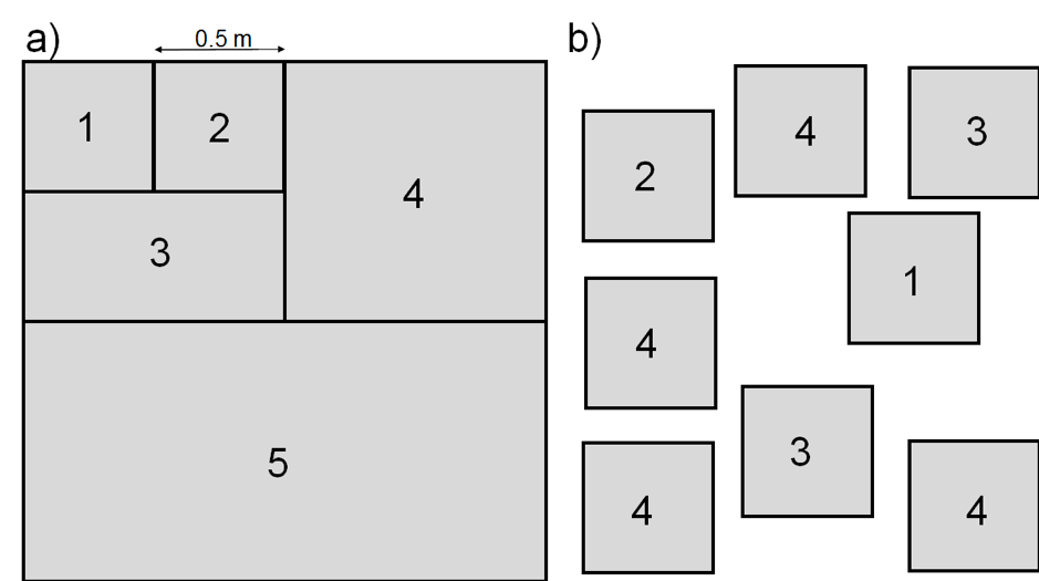
Plot size depends on plant community composition and plant size, and varies systematically across vegetation types (Smart et al., 2017, Supporting documentation). An appropriate plot size may be determined using a nested plot design (Figure 2.1.1.1 a) or a multi-plot approach (Figure 2.1.1.1 b). The number of plant species is determined in plots of doubling sizes (1 to 4 doubling steps, or more). The suggested minimum plot size is when the percentage increase in plant species is lower than 10% when the plot size is doubled. Often, this method results in plot sizes that are impractical to sample (because they are too large); the plot size may then be reduced to reflect 80% of the species, or 90% of the most productive species present. Commonly used dimensions for AGB observation plots are listed in Table 2.1.1.1. The number of replicated plots should reflect the observed heterogeneity in plant composition in the studied ecosystem. The more homogeneous the area is, the smaller the AGB observation plots can be (Traxler, 1997).

In forests, plot size depends on tree size. Variable radius plots are often used, where the plot size increases as a function of tree diameter, increasing the sample size for the large trees that most influence the biomass (Monserud & Marshall, 1999).

Table 2.1.1.1 General guidelines for the size of AGB observation plots.

Ecosystem	Dimension of area (m*m)	References
Temperate forest – tree layer	10 x 10 to 50 x 50	Traxler, 1997
Tropical forest and savanna – tree layer	20 x 20 to 100 x 100	Alder & Synnot, 1992
Forest – understorey	subplots of 1 x 1 to 2 x 2	Traxler, 1997
Shrubland	4 x 4 to 10 x 10	Traxler, 1997
Heathland	2 x 2 to 4 x 4	Traxler, 1997
Moor	0.1 x 0.1 to 1 x 1	Traxler, 1997
Grassland, savannah and alpine/arctic vegetation – grass layer	0.25 x 0.25 to 1 x 1	Bertora et al., 2012; Linstädter & Ruppert, 2015

 

 

AGB observation plots should be permanent and marked. Aluminium tubes or other metal tags at each corner are recommended. In study sites where visible plot markers may be stolen or removed (such as experimental sites in the Global South where the market price of aluminium or other metals may provoke theft), we recommend a combination of aboveground with belowground tags. For aboveground tags, materials with a low market price such as plastic sticks are most feasible. For belowground tags, we recommend magnets (buried to a depth of 15–25 cm); these are retrievable with a magnet detector. If the area is subject to unpredictable soil compaction (e.g. through frost or heavy machines), retrieval of magnets can be very difficult. For larger experiments, a GPS reading of plot corners, preferably with a differential GPS, is an alternative. Marking plots may be problematic in, for example, grazed ecosystems where permanent structures may increase the concentration of grazing animals and lead to preferential grazing within plots. In this case, Dodd (2011) may be consulted for alternative plot-relocating methods (see Special cases below).

 

Measuring AGB

Destructive harvesting is generally a more accurate estimate of AGB than a non-destructive AGB assessment. However, repeated non-destructive estimates of AGB are preferred in manipulation experiments (e.g. Kongstad et al., 2012; Tielbörger et al., 2014) if cutting or grazing is not part of the disturbance regime of the studied ecosystem. Non-destructive proxies of AGB can normally be measured with a little training, but measurements are time-consuming. Field spectroscopy requires more elaborate (technical) skills, and can be hampered by difficult external requirements such as unfavourable weather/cloud conditions in tropical environments (Ferner et al., 2015).

The methods described below are divided into 1) non-forest AGB methods and 2) forest AGB methods. Shrublands may fall into either of these two categories. In non-forest ecosystems (low-vegetation such as agriculture, grasslands, shrublands, etc.), the most frequently used non-destructive AGB methods are 1) point-intercept method (Goodall, 1952; Jonasson, 1988; Damgaard et al., 2009; Hudson & Henty et al., 2009; Valolahti et al., 2015), 2) field spectroscopy (Pearson et al., 1976; Milton et al., 2009; Ferner et al., 2015), and 3) visual cover estimation (Braun-Blanquet, 1932; Sykes et al., 1983; Peet et al., 1998). These methods require a destructive harvest outside the experimental area to obtain AGB estimates from the non-destructive vegetation assessments. Comparisons of methods show that each of the above methods can be effective in estimating AGB (Onodi et al., 2017a).

 

Measuring AGB in agriculture, grasslands, and shrublands (non-forests) (Gold standard)

• a) Destructive harvesting (Bertora et al., 2012). AGB that is rooted within the AGB observation plots is harvested by clipping the vegetation homogeneously above (e.g. 2 cm) the soil surface except if the vegetation includes substantial amounts of rosette-plants or includes aboveground stolens. Slow-growing, small vegetation (e.g. in alpine/arctic ecosystems) may be cut homogeneously closer to the soil surface (e.g. 0.5 cm). For shrubs rooted within the observation plots, leaves and the current year’s woody growth should be collected. If woody vegetation is part of the plot, a mixture between the gold and bronze standard can be used to assess AGB of grass vegetation (destructive harvest) and shurbs (non-destructive harvest, see below). The timing of sampling depends on the vegetation type and land-use practice. For further details see Timing of sampling Destructive harvesting is suggested for:
• agricultural and managed ecosystems where the harvest is part of the management practice
• herbaceous-dominated ecosystems (NutNet protocol): AGB that is rooted in parts of the observation plots may be harvested destructively over time (NutNet protocol). For example, if AGB is monitored over four years, 25% of the AGB observation plot can be harvested each year
• manipulation plots that simulate grazing (Linstädter & Ruppert, 2015)
• the end of an experiment.

Harvested AGB is then sorted into live and dead biomass, growth form, species, and plant organs when the plant material is still wet (Table 2.1.1.2). After sorting, plant material is dried at 65 ^oC to constant weight. AGB is calculated by summing up all the dry-weight fractions and is expressed in grams of dry biomass per m².

Table 2.1.1.2 Hierarchy of detail documented for plant material from destructive harvests. (Fresh) Plant material should, at the minimum, be divided into living, dead, and morbid structures of the different plant functional types. Species information is good to collect. Ideal is information on plant organs (Bertora et al., 2012; INCREASE).

Recommended		Good to have	Nice to have
Alive	Bryophytes/lichens	Species	location (soil surface/stem)
	Grasses		grasses/sedges/rushes
	Forbs		leaves/flowers
	Woody (shrubs)		stem/leaves/flowers
	Woody (trees)		current year’s woody growth
Dead	Grasses	Species	leaves/flowers
	Forbs		stem/leaves/flowers
	Woody		current year’s woody growth

 

4. b) Non-destructive point-intercept method (Goodall, 1952; Jonasson, 1988; also see 8 Plant community composition). The point-intercept method provides detailed information about plant community composition, 3-D canopy structure, reproduction, survival, mortality, community development, and plant competition (Jonasson, 1988; Damgaard et al., 2009; Kongstad et al., 2012). The assessment of dead and living plant parts can be used to estimate litter production of grassland species where litter remains attached to the plants (‘standing dead matter’).

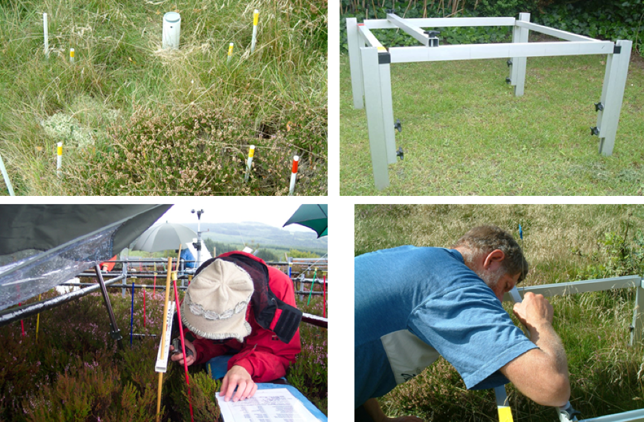
To use the point-intercept method, the AGB observation plot is divided into a reference grid by using a mountable frame above the plant canopy (Picture 2.1.1.2). The four corners of the frame need to be permanently marked. At each grid point, a pin is lowered vertically through the vegetation. For each plant hit along the pin, height and plant species are recorded (field notes or dictaphone). The hits of all species and plant organs (flower, annual shoot), status (alive, dead), and height are documented. Measurement protocols are detailed in the INCREASE protocol (INCREASE, 2014). It is also common to do a 2-D recording without height of pin hits on species. It is very fast but provides only plant cover estimates and is not suitable for converting pin-hits to biomass (see AGB conversion to Aboveground Net Primary Production below).

To convert pin-hits surveyed in the AGB observation plots to actual AGB, vegetation plots of the same size and the same vegetation composition have to be surveyed outside the experimental area. After surveying these reference plots, AGB (and optionally BGB) is harvested and sorted, and dry AGB is determined (see Destructive harvest above). We suggest surveying a minimum of ten representative vegetation plots outside the experimental area. If the vegetation at your site is heterogeneous, the calibration should be performed for different vegetation compositions. Reference surveys outside the experimental or observation plots need to be repeated with time when a change in vegetation has occurred, for example after pest outbreaks and vegetation responses to experimental treatments (Onodi et al., 2017b).

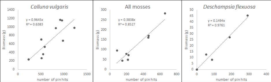
For each survey plot, the total number of hits for each species on the pin is expressed as a proportion of all pin-hits in a plot. The proportions of species pin-hits are then correlated with the determined dry plant biomass (Figure 2.1.1.2, INCREASE, 2014). The derived relationship for each species is used to convert pin-hits measured in the AGB observation plots to biomass per area. The total AGB in each AGB observation plot equals the sum of biomass of all species; AGB needs to be expressed per m². If the vegetation surveys are carried out at the same time of year for consecutive years, these measures of AGB can be used to estimate ANPP (see section Special cases below).

 

 

Measuring AGB in agriculture, grasslands, and shrublands (non-forests) (Bronze standards)

The ‘’Normalized Differential Vegetation Index’’ (NDVI) and visual estimation cover estimates are both proxies of AGB and need to be converted to AGB values by using measurements of destructive harvests outside the experimental area as described for the gold standard.

 

1. a) NDVI (Pearson et al., 1976; Milton et al., 2009). The most frequently used proxy for AGB is the NDVI (Tucker, 1979) which correlates with green AGB (Tucker & Sellers, 1986; Ferner et al., 2015). It is the quickest method to assess the living green biomass (Onodi et al., 2017b) and is a good measure to track seasonal changes within the green plant biomass (Gamon et al., 1995). Using a portable multi-spectral radiometer, incoming and reflected light intensity is measured at different wavebands in each AGB observation plot. The weather conditions need to be recorded as precisely as possible and date and time are crucial information. Uniform overcast without direct radiation is the preferred condition during measurements (Bertora et al., 2012), although newer equipment is able to account for changes in light intensity. We advise reading the manual of your equipment carefully.

An NDVI sensor can be hand-held or mounted on a boom above the AGB observation plots. The sensor needs to be placed higher above the canopy the larger the AGB observation plot is to capture the entire biomass within the plot. For example, Onodi et al. (2017b) levelled an NDVI sensor 1.8 m above a 0.25 m² plot and 2.8 m above a 1 m² plot. The use of a boom reduces the interference of the operator with the measurements. Multispectral radiometers are usually composed of paired sensors for NIR₈₁₀ and R₆₆₀ and both wavebands can be measured simultaneously (INCREASE, 2014). Using a spectrometer with sensors for both incoming and reflected light provides a more robust result and is thus not dependent on a clear sky (INCREASE, 2014).

NDVI is calculated as NDVI = (NIR₈₁₀ − R₆₆₀) / (NIR₈₁₀ + R₆₆₀), where NIR₈₁₀ is the reflectance measured at the near-infrared (NIR) waveband (centred at 810 nm) and R₆₆₀ is the reflectance measured at the red (R) waveband (660 nm). Note that NDVI goes to saturation at high canopy density and thus is less effective when vegetation becomes dense (leaf area index (LAI) above 2) (Gamon et al., 1995).

4. b) Visual cover estimation (Braun-Blanquet, 1932; Sykes et al., 1983; Peet et al., 1998). It has been historically used to assess the plant community composition of an ecosystem (see protocol 4.8 Plant community composition). Visual cover estimation can also be used to estimate AGB in climate-change experiments (Zhang & Welker, 1996; Tielbörger et al., 2014). Percentage cover is typically estimated as 25%, 30%, 35% etc. above 20% cover, full numbers between 2% and 20%, and to one decimal digit when cover is below 2%, i.e. 1.5% or 0.4% (Ónodi et al., 2017a). In case of multiple observers, training may be needed to facilitate consistency (Sykes et al., 1983). Based on calibration in plots with destructive sampling, the estimated cover can be converted to AGB. It has been shown that visual cover estimation can be similar in accuracy to field spectroscopy and the point-intercept method in estimating AGB (Ónodi et al., 2017a, 2017b).

 

Measuring AGB in forests (Gold standard)

In forests, AGB can be estimated using allometric relationships, which use simple measures of diameter, and sometimes other variables, to estimate more complex variables, such as leaf biomass. The commonly used model is a power form equation (A = αB^x + … +βZ^y), with coefficients derived from empirical measurements. Often the equation form is simplified to A= aD^x, where D is the tree diameter. Because allometric equations can vary considerably (Ketterings et al., 2001), the gold standard uses site-specific allometric equations for each species.

Several alternatives have been suggested to improve precision and generality. Chave et al. (2014) show that at least three tree parameters are needed to calculate robust, general allometric equations: 1) maximum tree height, 2) diameter at breast height (DBH), and 3) wood specific gravity. Monserud & Marshall (1999) also accounted for height to the base of the crown and competition indices, which account for differences in tree shape with variable stand density. Ketterings et al. (2001) use a function of tree height and wood density to parameterise across a range of sites, generalising their equations such that site-specific equations were no longer necessary.

To drive allometric equations, the following predictor variables are often required:

1. Maximum tree height is measured through trigonometric methods using laser equipment or mechanically with a telescopic stick with decimetre marks (Pérez-Harguindeguy et al., 2013).
2. DBH is defined as diameter at a height of 1.3 m. It is best measured using a laser relascope, callipers, or a DBH-tape. In case of buttresses or forked stems occurring above or below 1.3 m, DBH is measured just above the buttresses or below the fork. (Hoover, 2008; Avery & Burkhart, 2015).

Dendrometers are used to measure changes in stem size in a single radius, across the diameter or around the circumference of a stem at a particular height. For within-season measurements of changes in stem diameter or radius, both manual and automatic methods are available (Drew & Downes, 2009). Stainless steel band dendrometers, installed at breast height, can be used to determine the onset and cessation of diameter growth, as well as the seasonal variations in growth. The measurements can be made manually using digital callipers, but there are also band dendrometers with automatic recording. Point dendrometers can measure the changes in stem, branch, or coarse root radii with a resolution of less than 1 µm. At such high resolution, diurnal swelling and shrinking of the stem can be seen (Zweifel & Häsler, 2001). These stem radius changes consist of actual radial growth and shrinkage and swelling from the inflow and outflow of water (cf. Zweifel et al., 2006).

1. Wood specific gravity is measured as oven dry biomass divided by fresh volume. Biomass for this measurement is obtained by taking a wood core at breast height using an increment corer, aiming for the pith of the tree. Fresh volume is calculated from the core cylinder with length measured immediately after sampling the core and removing the bark and diameter defined by the increment corer (Williamson & Wiemann, 2010; Pérez-Harguindeguy et al., 2013). Data can also be taken from databases such as TRY (Kattge et al., 2011), DRYAD (Zanne et al., 2009), and BAAD (Falster et al., 2015).

A European database has been developed by Zianis et al. (2005), while Forrester et al. (2017) developed one for North American tree species. Jenkins et al. (2003) provide allometric equations, and Chave et al. (2014) provide a generic model for tropical forest trees. The international platform GlobAllomeTree can be consulted for different tree allometric equations (see Henry et al., 2013 and references therein). Allometric relationships are derived from a subset of trees. AGB observation plots often relate to one tree or a smaller group of surrounding trees. Trees have to be marked or exact coordinates are needed. Guidelines on the selection of trees can be found in Smart et al. (2017) and Bertora et al. (2012).

Allometric equations are highly species specific and thus accommodate species-specific and individual responses to climate manipulation. The use of published allometric relationships for a species may be suitable if the development of AGB over time is of interest because the incremental change in AGB over a given time rather than the actual measure of AGB is the information of interest. However, if the environmental conditions between years are very different and the responses of trees to these conditions change, the desired information in AGB may be hidden in the “noise” introduced by using non-specific allometric relationships (Coomes & Allen, 2007).

If AGB of small forest stands or individual trees is of interest, we suggest building allometric relationships from nearby trees of the species of interest (see Bertora et al., 2012 for guidelines). The building of allometric relationships requires either the sampling of branches or the felling of trees (Monserud & Marshall, 1999), and the actual measurement of weight, DBH, and wood density. If such sampling is not possible, a protocol involving tree coring and seasonal litter sampling as introduced in Smart et al. (2017, supplementary material) is preferred over the use of general allometric relationships found in the literature.

 

Handling and storage of AGB (Gold standard)

Plant material should be stored in a cool place if no oven is immediately available as metabolic processes can continue. All plant material is dried at a maximum of 70 ^oC for 72 h to constant weight. Dried plant material shall be stored in a desiccator during cooling down to prevent the dried material taking up air humidity. Dried and cooled plant material is weighed to the nearest 0.01 grams. AGB is expressed as weight of dry matter per unit area (g AGB m^-2).

There is no clear rule, what the optimal temperature for drying biomass is. Drying temperatures range from 50 – 80 °C (NutNet protocol; Milner & Elfyn Hughes, 1970; Pérez-Harguindeguy et al., 2013). Dependent on the plant material (fleshyness, thickness), the time plant material needs to dry to constant weight varies. Too high temperatures can change components in the plant (e.g. damage secondary compounds, carbon compounds), which will affect the biomass. Contrary, if biomass is dried at too low temperature (50 – 60 °C), metabolic processes may continue during the drying process or can trigger a stress reaction in the plant. In both cases this will affect the biomass of the plant.

Dried AGB can either be stored in paper bags, or stored frozen in plastic bags. The latter is more convenient if samples are to be sorted into different fractions. If possible, dried material is measured for carbon and nutrient content.

 

Where to start

Chave et al. (2014), Damgaard (2014), Fahey & Knapp (2007)

 

2.1.1.2 Special cases, emerging issues, and challenges

1. a) Special case: AGB sampling in grazed systems

To measure AGB in grazed systems, the gold standard is the “moveable exclosure” (ME) method (McNaughton et al., 1996; Knapp et al., 2012). It implies a paired plot design, where grazed study plots are combined with adjacent ME plots. The paired plots are moved one to several times per year. The movement frequency and the repeated sampling of plant biomass should reflect both the intensity of herbivory and plant re-growth rates (McNaughton et al., 1996); in semi-arid environments, monthly time intervals during the growing season have been used (Knapp et al., 2012). Prior to randomly moving the paired plots to a new location within the treatment area, AGB is harvested both on the ME plots (or from a smaller area within the ME) and on the adjacent grazed plot. In this special case, ANPP can be calculated from AGB harvested in ME plots (see below) while the AGB from grazed plots is used to estimate grazing offtake (Linstädter & Ruppert, 2015).

The bronze standard for measuring AGB under grazed conditions is the “clipping method”. Grazing exclosure cages are left in the field preventing actual grazing. Vegetation in exclosure cages is simulated via clipping, with the end-of-season standing crop also being clipped (McNaughton et al., 1996). The clipping method can mimic grazing if livestock grazing is not possible, for example due to small size of treatment plots (Linstädter & Ruppert, 2015).

1. b) Timing of sampling

Sampling can be done at different times during the season to address different ecological questions. We advise that sampling dates are not fixed but are flexible to accommodate the phenological stage of the plants, and matched with management practice if necessary. Moreover, biomass sampling has to be attuned to vegetation characteristics (herbaceous v. non-herbaceous, patchy v. non-patchy), and to the seasonality of the ecosystem (Linstädter & Ruppert, 2015). To quantify maximum biomass, AGB is often sampled at peak growing only (NutNet protocol; Linstädter & Ruppert, 2015). To quantify sequential growth, biomass is harvested at several times during the growing season (Scurlock et al., 2002). This “repeated sampling” is the gold standard for systems with a marked seasonality, and particularly for systems with high biomass turnover rates, such as temperate and humid environments (Scurlock et al., 2002; Ruppert & Linstädter, 2014).

1. c) Standing and attached dead biomass

The term “biomass” may be defined to include standing dead trees and dead branches on live trees. Dead branches can be assessed using standard procedures (Monserud & Marshall, 1999). However, because they may lack small branches and foliage, standing dead trees often require different model forms and parameterisation (Powers et al., 2013). In either case, dead trees and branches must be treated carefully because they can represent a significant biomass pool.

1. d) AGB conversion to Aboveground Net Primary Production (ANPP, grams of biomass per m² per year)

The method used to convert AGB measurements to ANPP should reflect the AGB estimation method, i.e. if AGB was harvested several times during the growth period, ANPP is estimated with “incremental methods”, which sum the seasonal accumulation of biomass (Ruppert & Linstädter, 2014; see Scurlock et al., 2002 for details on the protocols). We suggest the use of Smalley’s method (the sum of positive increments in live and recent dead biomass; Method 5 in Scurlock et al., 2002) for ecosystems and experiments where biomass can be destructively harvested as it is a good compromise between accuracy and sampling effort.

Alternatively, AGB can be converted to ANPP using the sum of positive increments in living biomass only (Method 4 in Scurlock et al., 2002). This method is similar to AGB conversions to ANPP that are used for non-destructive estimations of green AGB (see above). As AGB from non-destructive measurements is performed at peak growing season, the conversion of AGB into ANPP can be done with a “peak method” that uses single biomass measurements at peak biomass conditions (Ruppert & Linstädter, 2014; see Scurlock et al., 2002 for details on the protocols). Among these peak methods, “peak standing crop” (live plus recent dead biomass) is the gold standard. To calculate ANPP using the peak method, AGB estimates from two consecutive years are needed to calculate ANPP as:

ANPP (g biomass m^-2 yr^-1) = AGB_{year x} – AGB_{year x-1}

For annual plants, AGB equals ANPP. For perennial plants, including trees, a carbon-budget approach is necessary. Such an approach estimates ANPP from:

ANPP = Change in aboveground biomass + mortality + litterfall

An alternative is to focus on woody ANPP, which allows one to use the change in biomass estimated from allometrics (Gough et al., 2013), but it remains necessary to account for any mortality that may have occurred.

2. e) Light Detection And Ranging (LIDAR), can be used to derive biome specific AGB estimates (for details see protocol 2.3.3 Upscaling from the plot scale to the ecosystem and beyond).

 

2.1.1.3 References

Theory, significance, and large datasets

Henry et al. (2013), Kattge et al. (2011)

 

More on methods and existing protocols

Beierkuhnlein (2006), Bertora et al. (2012), Mueller-Dombois & Ellenberg (1974), NutNet protocol, Scurlock et al. (2002)

 

All references

Addo-Danso, S. D., Prescott, C. E., & Smith, A. R. (2016). Methods for estimating root biomass and production in forest and woodland ecosystem carbon studies: A review. Forest Ecology and Management, 359, 332-351.

Alder, D., & Synnott, T. J. (1992). Permanent Sample Plot Techniques for Mixed Tropical Forest. Oxford Forestry Institute, University of Oxford.

Avery, T. E., & Burkhart, H. E. (2015). Forest Measurements. Waveland Press.

Beierkuhnlein, C. (2006). Biogeography. Stuttgart, Germany: Ulmer Verlag.

Bertora, C., Blankman, D., Vedove, G. D., Firbank, L., Frenzel, M., Grignani, C., … Stadler, J. (2012). Manual: “Handbook for Standardised Ecosystem Protocols”, http://expeeronline.eu/images/ExpeER-Documents/Handbook_of_standardized_ecosystem_protocols.pdf

Braun-Blanquet, J. (1932). Plant Sociology. The Study of Plant Communities. New York: McGraw-Hill.

Chave, J., Réjou-Méchain, M., Búrquez, A., Chidumayo, E., Colgan, M. S., Delitti, W. B. C., … Vieilledent, G. (2014). Improved allometric models to estimate the aboveground biomass of tropical trees. Global Change Biology, 20, 3177-3190.

Clark, D. A., Brown, S., Kicklighter, D. W., Chambers, J. Q., Thomlinson, J. R., & Ni, J. (2001). Measuring net primary production in forests: concepts and field methods. Ecological Applications, 11(2), 356-370.

Cleveland, C. C., Townsend, A. R., Taylor, P., Alvarez-Clare, S., Bustamante, M. M. C., Chuyong, G., … Wieder, W. R. (2011). Relationships among net primary productivity, nutrients and climate in tropical rain forest: a pan-tropical analysis. Ecology Letters, 14, 939-947.

Coomes, D. A., & Allen, R. B. (2007). Effects of size, competition and altitude on tree growth. Journal of Ecology, 95, 1084-1097.

Damgaard, C. (2014). Estimating mean plant cover from different types of cover data: a coherent statistical framework. Ecosphere, 5(2), 1-7.

Damgaard, C., Riis-Nielsen, T., & Schmidt, I. K. (2009). Estimating plant competition coefficients and predicting community dynamics from non-destructive pin-point data: a case study with Calluna vulgaris and Deschampsia flexuosa. Plant Ecology, 201, 687-697.

Dodd, M. (2011). Where are my quadrats? Positional accuracy in fieldwork. Methods in Ecology and Evolution, 2(6), 576-584.

Domínguez, M. T., Sowerby, A., Smith, A. R., Robinson, D. A., Van Baarsel, S., Mills, R. T., … & Emmett, B. A. (2015). Sustained impact of drought on wet shrublands mediated by soil physical changes. Biogeochemistry, 122(2-3), 151-163.

Drew, D. A., & Downes, G. M. (2009). The use of precision dendrometers in research on daily stem size and wood property variation: A review. Dendrochronologia, 27, 159-172.

Fahey, T. J., & Knapp, A. K. (Eds.). (2007). Principles and Standards for Measuring Primary Production.  Oxford: Oxford University Press.

Falster, D. S., Duursma, R. A., Ishihara, M. I., Barneche, D. R., FitzJohn, R. G., Vårhammar, A., … Baltzer, J. L. (2015). BAAD: a Biomass And Allometry Database for woody plants. Ecology, 96(5), 1445-1445.

Ferner, J., Linstädter, A., Südekum, K.-H., & Schmidtlein, S. (2015). Spectral indicators of forage quality in West Africa’s tropical savannas. International Journal of Applied Earth Observation and Geoinformation, 41, 99-106.

Forrester, D. I., Tachauer, I. H. H., Annighoefer, P., Barbeito, I., Pretzsch, H., Ruiz-Peinado, R., … Saha, S. (2017). Generalized biomass and leaf area allometric equations for European tree species incorporating stand structure, tree age and climate. Forest Ecology and Management, 396, 160-175.

Gamon, J. A., Field, C. B., Goulden, M. L., Griffin, K. L., Hartley, A. E., Joel, G., … Valentini, R. (1995). Relationships between NDVI, canopy structure, and photosynthesis in three Californian vegetation types. Ecological Applications, 5, 28-41.

Goodall, D. W. (1952) Some considerations in the use of point quadrats for the analysis of vegetation. Australian Journal of Biological Sciences, 5(1), 1-41.

Gough, C. M., Hardiman, B. S., Nave, L. E., Bohrer, G., Maurer, K. D., Vogel, C. S., … Curtis, P. S. (2013). Sustained carbon uptake and storage following moderate disturbance in a Great Lakes forest. Ecological Applications, 23(5), 1202-1215.

Grayston, S. J., Vaughan, D., & Jones, D. (1997). Rhizosphere carbon flow in trees, in comparison with annual plants: the importance of root exudation and its impact on microbial activity and nutrient availability. Applied Soil Ecology, 5(1), 29-56.

Henry, M., Bombelli, A., Trotta, C., Alessandrini, A., Birigazzi, L., Sola, G., … Valentini, R. (2013). GlobAllomeTree: international platform for tree allometric equations to support volume, biomass and carbon assessment. Iforest – Biogeosciences and Forestry, 6, 326.

Hoover, C. M. (Ed.). (2008). Field Measurements for Forest Carbon Monitoring: A Landscape-scale Approach. Springer Science & Business Media.

Hudson, J. M. G., & Henry, G. H. R. (2009). Increased plant biomass in a High Arctic heath community from 1981 to 2008. Ecology, 90(10), 2657-2663.

INCREASE (2014). – An integrated network on climate change activities on shrubland ecosystems: final report. Schmidt IK, Larsen KS, Ransijn J, Arndal MF, Tietema A, De Angelis P, Duce P, Cesaraccio C, Zara P, Spano D, Mereu S, Kröel-Dulay G, Smith A, Emmett B, Jones D, Lellei-Kovács E, De Dato G, Guidolotti G. Department of Geosciences and Natural Resource Management, University of Copenhagen. www.increase.ku.dk

Jenkins, J. C., Chojnacky, D. C., Heath, L. S., & Birdsey, R. A. (2003). National-scale biomass estimators for United States tree species. Forest Science, 49(1), 12-35.

Jonasson, S. (1988). Evaluation of the point intercept method for the estimation of plant biomass. Oikos, 52, 101-106.

Kattge, J., Diaz, S., Lavorel, S., Prentice, I. C., Leadley, P., Bönisch, G., … Wright, I. J. (2011). TRY – a global database of plant traits. Global Change Biology, 17, 2905-2935.

Ketterings, Q. M., Coe, R., van Noordwijk, M., Ambagau’, Y., & Palm, C. A. (2001). Reducing uncertainty in the use of allometric biomass equations for predicting above-ground tree biomass in mixed secondary forests. Forest Ecology and Management, 146(1), 199-209.

Knapp, A. K., Hoover, D. L., Blair, J. M., Buis, G., Burkepile, D. E., Chamberlain, A., … Blake, D. (2012). A test of two mechanisms proposed to optimize grassland aboveground primary productivity in response to grazing. Journal of Plant Ecology, 5(4), 357-365.

Kongstad, J., Schmidt, I. K., Riis-Nielsen, T., Arndal, M. F., Mikkelsen, T. N., & Beier, C. (2012). High resilience in heathland plants to changes in temperature, drought, and CO₂ in combination: results from the CLIMAITE experiment. Ecosystems, 15, 269-283.

Kuzyakov, Y., & Domanski, G. (2000). Carbon input by plants into the soil. Review. Journal of Plant Nutrition and Soil Science, 163(4), 421-431.

Lauenroth, W. K., & Sala, O. E. (1992). Long-term forage production of North American shortgrass steppe. Ecological Applications, 2, 397-403.

Linstädter, A., & Ruppert, J. C. (2015). Add on protocol to the international drought experiment (IDE): studying combined effects of drought & grazing (‘Drought Act’). http://www.ag-linstaedter.botanik.uni-koeln.de/sites/ag_linstaedter/user_upload/Drought-Net_Grazing_Add-On_Protocol.pdf

Martin, R., Müller, B., Linstädter, A., & Frank, K. (2014). How much climate change can pastoral livelihoods tolerate? Modelling rangeland use and evaluating risk. Global Environmental Change, 24, 183-192.

McNaughton, S. J., Milchunas, D. G., & Frank, D. A. (1996). How can net primary productivity be measured in grazing ecosystems? Ecology, 77(3), 974-977.

Milner, C., & Elfyn Hughes, R. (1968) Methods for the Measurement of the Primary Production of Grassland. IBP Handbook 6, Oxford.

Milton, E. J., Schaepman, M. E., Anderson, K., Kneubühler, M., & Fox, N. (2009). Progress in field spectroscopy. Remote Sensing of the Environment, Imaging Spectroscopy Special Issue, 113, Supplement 1: S92-S109.

Mokany, K., Raison, R., & Prokushkin, A. S. (2006). Critical analysis of root:shoot ratios in terrestrial biomes. Global Change Biology, 12(1), 84-96.

Monserud, R. A., & Marshall, J. D. (1999). Allometric crown relations in three northern Idaho conifer species. Canadian Journal of Forest Research, 29(5), 521-535.

Mueller-Dombois, D. & Ellenberg, H. (1974). Aims and Methods of Vegetation Ecology. New York: John Wiley & Sons.

NutNet protocol: http://www.nutnet.umn.edu/exp_protocol, Accessed 04 March 2018

Ónodi, G., Kertész, M., Kovács-Láng, E., Ódor, P., Botta-Dukát, Z., Lhotsky, B., … Kröel-Dulay, G., (2017a). Estimating aboveground herbaceous plant biomass via proxies: The confounding effects of sampling year and precipitation. Ecological Indicators, 79, 355-360.

Ónodi, G., Kröel-Dulay, G., Kovács-Láng, E., Ódor, P., Botta-Dukát, Z., Lhotsky, B., … Kertész, M. (2017b). Comparing the accuracy of three non-destructive methods in estimating aboveground plant biomass. Community Ecology, 18, 56-62.

Pearson, R. L., Miller, L. D., & Tucker, C. J. (1976). Hand-held spectral radiometer to estimate gramineous biomass. Applied Optics, 15, 416-418.

Peet, R. K., Wentworth, T. R., & White, P. S. (1998). A flexible, multi-purpose method for recording vegetation composition and structure. Castanea, 63, 262-274.

Pérez-Harguindeguy, N., Díaz, S., Garnier, E., Lavorel, S., Poorter, H., Jaureguiberry, P., … Cornelissen, J. H. C. (2013). New handbook for standardised measurement of plant functional traits worldwide. Australian Journal of Botany, 61(3), 167-234.

Powers, E. M., Marshall, J. D., Zhang, J., & Wei, L. (2013). Post-fire management regimes affect carbon sequestration and storage in a Sierra Nevada mixed conifer forest. Forest Ecology and Management, 291, 268-277.

Ruppert, J. C., & Linstädter, A. (2014). Convergence between ANPP estimation methods in grasslands – A practical solution to the comparability dilemma. Ecological Indicators, 36, 524-531.

Ruppert, J. C., Harmoney, K., Henkin, Z., Snyman, H. A., Sternberg, M., Williams, W., & Linstädter, A., (2015). Quantifying drylands’ drought resistance and recovery: The importance of drought intensity, dominant life history and grazing regime. Global Change Biology, 21, 258-1270.

Scheiter, S., Langan, L., & Higgins, S. I. (2013). Next-generation dynamic global vegetation models: learning from community ecology. New Phytologist, 198, 957-969.

Scurlock, J. M. O., Johnson, K., & Olson, R. J. (2002). Estimating net primary productivity from grassland biomass dynamics measurements. Global Change Biology, 8, 736-753.

Singh, J. S., Lauenroth, W. K., & Steinhorst, R. K. (1975). Review and assessment of various techniques for estimating net aerial primary production in grasslands from harvest data. Botanical Review, 41, 181-232.

Smart, S. M., Reinsch, S., Mercado, L., Blanes, M. C., Cosby, B. J., Glanville, H. C., … Emmett, B. A. (2017). Plant aboveground and belowground standing biomass measurements in the Conwy catchment in North Wales (2013 and 2014). NERC Environmental Information Data Centre. doi: 10.5285/46bb0117-ed5d-4167-a375-d84d1237cf21

Sykes, J. M., Horrill, A. D., & Mountford, M. D. (1983). Use of visual cover assessments as quantitative estimators of some British woodland taxa. Journal of Ecology, 71, 437-450.

Tielbörger, K., Bilton, M. C., Metz, J., Kigel, J., Holzapfel, C., Lebrija-Trejos, E., … Sternberg, M. (2014). Middle-Eastern plant communities tolerate 9 years of drought in a multi-site climate manipulation experiment. Nature Communications, 5, 5102.

Traxler, A. (1997).  Handbuch des vegetationsökologischen Monitorings: Methoden, Praxis, angewandte Projekte. Teil A: Methoden. Bundesministerium für Umwelt, Jugend und Familie, Wien, Austria. http://www.umweltbundesamt.at/fileadmin/site/publikationen/M089A.pdf

Tucker, C. J. (1979). Red and photographic infrared linear combinations for monitoring vegetation. Remote Sensing of Environment, 8(2), 127-150.

Tucker, C. J., & Sellers, P. J. (1986). Satellite remote sensing of primary production. International Journal of Applied Earth Observation and Geoinformation, 7, 1395-1416.

Valolahti, H., Kivimäenpää, M., Faubert, P., Michelsen, A., & Rinnan, R. (2015). Climate change-induced vegetation change as a driver of increased subarctic biogenic volatile organic compound emissions. Global Change Biology, 21, 3478-3488.

Williamson, G. B., & Wiemann, M. C. (2010). Measuring wood specific gravity… correctly. American Journal of Botany, 97(3), 519-524.

Younginger, B. S., Sirová, D., Cruzan, M. B., & Ballhorn, D. J. (2017). Is biomass a reliable estimate of plant fitness? Applications in Plant Sciences, 5(2), apps.1600094.

Zanne, A.E., Lopez-Gonzalez, G., Coomes, D. A., Ilic, J., Jansen, S., Lewis, S. L., & Miller, R. B. (2009). Global wood density database. doi: 10.5061/dryad.234

Zhang, Y., & Welker, J. M. (1996). Tibetan Alpine tundra responses to simulated changes in climate: aboveground biomass and community responses. Arctic & Alpine Research, 28, 203-209.

Zianis, D., Muukkonen, P., Mäkipää, R., & Mencuccini, M. (2005). Biomass and stem volume equations for tree species in Europe. Silva Fennica, 4, 1-63.

Zweifel, R., & Häsler, R. (2001). Dynamics of water storage in mature subalpine Picea abies: temporal and spatial patterns of change in stem radius. Tree Physiology, 21, 561-569.

Zweifel, R., Zimmerman, L., Zeugin, F., & Newbery, D. M. (2006). Intra-annual radial growth and water relations of trees: implication towards a growth mechanism. Journal of Experimental Botany, 57, 1445-1459.

 

 

Authors: Reinsch S¹, Linstädter A², Beil I³, Berauer B⁴, Kröel-Dulay G⁵, Stuart-Haëntjens E⁶, Schmidt IK⁷

Reviewers: Ruppert JC⁸, Kreyling J³, Linder S⁹, Marshall J¹⁰, Smart S¹¹, Weigel R¹²

 

Affiliations

¹ Centre for Ecology & Hydrology, Environment Centre Wales (ECW), Bangor, UK

² Institute of Crop Science and Resource Conservation (INRES), University of Bonn, Bonn, Germany

³ Experimental Plant Ecology, Institute of Botany and Landscape Ecology, University of Greifswald, Greifswald, Germany

⁴ Department of Disturbance Ecology, BayCEER, University of Bayreuth, Bayreuth, Germany

⁵ Institute of Ecology and Botany, MTA Centre for Ecological Research, Vácrátót, Hungary

⁶ Virginia Commonwealth University, Department of Biology, Richmond, USA

⁷ Department of Geosciences and Natural Resource Management, University of Copenhagen, Frederiksberg, Denmark

⁸ University of Tübingen, Plant Ecology, Institute of Evolution and Ecology, Auf der Morgenstelle 5, 72076 Tübingen, Germany

⁹ Swedish University of Agricultural Sciences, Southern Swedish Forest Research Centre, Alnarp, Sweden

¹⁰ Department of Forest Ecology and Management, Swedish University of Agricultural Sciences, Umeå, Sweden

¹¹ Environment Centre Lancaster, Library Avenue, Lancaster University, Lancaster, UK

¹² Plant Ecology, Albrecht-von-Haller Institute for Plant Sciences, University of Goettingen, Goettingen, Germany