Authors: Kreyling J1, Lembrechts JJ2, De Boeck HJ2
Reviewer: Lenz A3
Measurement unit: same as unit of interest, e.g. °C; Measurement scale: for frost tolerance: temperature test chamber; Equipment costs: €€€; Running costs: €; Installation effort: medium; Maintenance effort: low; Knowledge need: medium; Measurement mode: manual measurement
Our understanding of plant ecology hinges largely on studies exploring stress responses and explaining their specific mechanisms. Generally, stress has a physiological impact, leading to the loss of tissue or a severe restriction of physiological processes (Körner, 2012). Stress responses can be gradual (eustress) with slight deviations from a reference state, or destructive leading to severe damage and the loss of tissue. Stress has a direct physiological impact and is, as such, zonal, i.e. typically associated with environmental gradients, for instance elevation (Körner, 2012). Potential stress factors include deficiency and excess of light, UV-radiation, heat, cold, frost, or drought. Stress should not be confused with disturbance, which refers to a mechanical or physical impact on plants, such as wind, burial, grazing, trampling, or soil compaction. In light of climate change and other global changes, several stress factors are intensifying, leading to renewed interest in plant stress responses (Tylianakis et al., 2008). Stress responses are simply any plant reaction to any stress factor and can be measured by a multitude of response parameters and experimental or observational methods.
Generally, studies of stress responses range from the quantification of net effects at ecosystem level such as CO2-fluxes under contrasting expression of stress (Ciais et al., 2005) to detailed molecular physiological studies (Thomashow, 1999; Munns & Tester, 2008). Most studies focus on destructive stress, which can be experimentally investigated. Plant responses to destructive stress include “escape” and “resistance”. Escape is a temporal or spatial evasion of the stress, for example shedding green leaves in autumn, or keeping meristems belowground to escape freezing stress in winter. Resistance is further subdivided into avoidance and tolerance. Avoidance implies that the stress is avoided, for example by supercooling water to survive temperatures below 0 °C. To truly be able to survive temperate, boreal, and arctic climates, plants need to be able to tolerate freezing temperatures, i.e. the water freezes within the plant and the plant survives this freezing.
5.4.1 What and how to measure?
A widely used concept to quantify stress tolerance is the LD (lethal dose) approach adopted from toxicology (Trevan, 1927). The median lethal dose, LD50 (also called LC50 for lethal concentration or LCt50 for lethal concentration and time) of a given stress factor is the dose required to kill half the members of a tested population after a specified test duration. Here, its use in stress ecology is exemplified by referring to frost stress and determination of LT50, the median lethal temperature. LD50 for any other stress factor can be assessed accordingly.
Four ways of measuring LD50
Generally, we measure the survival of organisms or organs under controlled environmental conditions. The lethal dose is determined by regressing survival or quantitative performance of organisms or tissues against a gradient of increasing severity of a given stress factor under laboratory conditions. Ideally, the stress gradient should cover the full range from non-stressed to completely lethal conditions for the test subject, including a control at both ends. By fitting a model to the observed relation between survival and stress, the median lethal dose (LD50) is determined. The lethal temperature for 50% of the investigated population (LT50) can be determined for whole organisms or for specific plant organs such as flowers, leaves, roots, twigs, or buds. Survival or performance of the plants or of the specific organs can be determined by various methods. Here, only the measurement after simulating the stress is described. The methods to simulate the stress are described below under Installation, field operation, maintenance, interpretation.
a) Direct measurement of the stress response during induction of the stress. Cell damage can be directly quantified by differential thermal analysis (DTA). The exotherm reaction (warming peak when water freezes) of intracellular freezing (low temperature exotherm) is measured by miniature temperature thermocouples directly inserted into tissues (Räisänen et al., 2006; Pramsohler et al., 2012). The temperature of intracellular freezing is the lethal temperature of the sample. LT50 values can be calculated as the median of replicates. Comparing samples to dead tissue not showing any low temperature exotherm reaction upon intracellular freezing and putting the samples into aluminium blocks can improve the precision of the method considerably (Räisänen et al., 2006). Advantages: This method is the most direct method to measure freezing resistance. It is objective and provides a very quick and direct test that can even be applied in the field (Pramsohler et al., 2012). Disadvantages: DTA is not applicable for all organs and species (Salazar-Gutiérrez et al., 2016). Before use, pre-trials are recommended as the low temperature exotherms are not always detectable for particular species and tissue types. The technical equipment for this method is different from all other methods described here.
b) Continued monitoring under non-limiting conditions (Sakai, 1966). After freezing stress has been induced, whole plants or organs such as twigs with buds are kept under non-stressful conditions (e.g. above freezing temperatures) for a prolonged period of time, during which their performance is regularly monitored. Since death of whole plants or plant organs is usually hard to determine, testing for regrowth or sprouting after induction of the stress is a valuable option. Monitoring times depend on the studied organisms or organs. For frost tolerance of tree buds during winter for example, monitoring can continue until leaf unfolding, which is the ultimate measure of bud survival. Uninodal (Bilavčík et al., 2012) or longer twigs (Sakai, 1966) can be kept for weeks with their bases in water if the water is changed regularly, the base is freshly cut on a weekly basis, and the upper cut (for uninodal samples) is sealed with wax or paraffin. Advantages of this method are that it is easily applicable and death of investigated organs is very obvious. Disadvantages are the long duration needed to wait until death is apparent.
c) Visual inspection of damage immediately after the stress (e.g. Vitasse et al., 2014). For many organs and species, damage can be visually quantified immediately after stress exposure. Freezing damage becomes apparent by the texture, odour, and discolouration of tissues caused by the oxidation of polyphenols and the decompartmentalisation of the protoplast (Sakai & Larcher, 1987). The method works well with different plant tissues such as leaves (e.g. Lenz et al., 2013, Vitasse et al., 2014), twigs (Lindén et al., 1996), buds (Lenz et al., 2013), and roots (Kreyling et al., 2012). After an initial learning phase, the method is easily applicable to almost any tissue. Comparing the investigated sample with the dead and the alive controls allows for a correct assessment of survival. Advantages of the method are that different tissues can be assessed differentially at the same time. For instance, LT50 values of leaf primordia and phloem and xylem tissue can be assessed in one open cut bud. Disadvantages are that in some species and tissues, for instance buds of Tilia platyphyllos, visual inspection becomes very hard since changes between alive and dead tissues are very subtle. However, after some training the method should be applicable to most tissues of most species. Caution should be taken to blind the samples to the stress level used, when visually assessing damage.
d) Indirect measurements of cell damage by electrolyte leakage after the stress (Whitlow et al. 1992). Electrolyte leakage is a proxy for cell damage. Target tissues are placed in a vial with deionised water after stress has been induced. After a certain amount of time, when the leakage of electrolytes is complete (to be determined for the samples studied), electrical conductivity of the water is measured. Thereafter, samples are killed completely (usually by autoclaving the samples), with the aim of destroying all cells. After a second waiting period, electrical conductivity of the water is measured again, corresponding to the complete leakage of dead cells. Different methods are suggested to further process the data (see Lim et al., 1998). Relative electrolyte leakage is the first value after the stress, divided by the second value after killing the sample completely. Injury is relative electrolyte leakage standardised by the electrolyte leakage of the alive control. Adjusted injury is injury standardised by electrolyte leakage of the dead control. These values (relative electrolyte leakage, injury, adjusted injury) are then fit to non-linear models. The inflection point of the non-linear function corresponds to the calculated LT50 Advantages: objective and reasonably quick. Disadvantages: first, electrolyte leakage data give a bulk signal of all immersed tissues within the water solution. For instance, when a bud is frozen, the LT50 calculated by electrolyte leakage is influenced by the LT50 of leaf primordia and xylem and phloem tissue, with every organ having a different contribution. Second, fitting of non-linear functions to data is not trivial. The search for optimal starting parameters in the fitting procedure might be hard to impossible, which will lead to no data. Further, the non-linear functions are not symmetric. Thus, different functions will result in different LT50 values on the same data. In addition, standardising data differently (relative electrolyte leakage, injury, adjusted injury) again leads to more variety of LT50 values on the same data, decreasing the comparability of the method. Caution should be taken to exactly describe the method used, since a large variety is available.
An alternative method for photosynthetically active organs similar to electrolyte leakage is comparing chlorophyll fluorescence after frost to control levels (Clement & van Hasselt, 1996).
Where to start
Lim et al. (1998), Neuner & Hacker (2012), Sakai (1966), Sutinen et al. (1992), Trevan (1927), Vitasse et al. (2014), Whitlow et al. (1992)
Installation, field operation, maintenance, interpretation
To study freezing resistance, basically one or several freezers are needed. Commercial systems are available for differential thermal analysis, as well as for controlled freezing runs. Some laboratories developed their own systems, either for a controlled freezing in parallel in several freezers (Lenz et al., 2013), or for in situ freezing in several chambers (Buchner & Neuner, 2009). Here, we describe the method for controlled freezing runs in detail, excluding differential thermal analysis.
The general course of a freezing run consists of collecting samples in situ, bringing them to the lab, processing them as fast as possible, putting them into the freezers, running the freezing programme, and assessing freezing resistance. Some steps are more critical than others. The effect of transport to the lab has not, so far, been investigated. However, temperatures before freezing have a large effect on the freezing resistance of a plant (Lenz et al., 2016a). Thus, the temperature used should ideally not deviate from ambient temperatures. Most important is the freezing and re-warming ramp, as well as the duration of the target stress level. For the freezing ramp, caution should be taken to simulate the conditions one would like to study as naturally as possible in the laboratory. For instance, if the lethal temperature under clear sky conditions in winter are of interest, when temperatures drop below freezing by radiative cooling, slow cooling rates of <5 K h-1 should be chosen. Immediate exposure to freezing temperatures can cause artefacts, for example by supercooling due to too drastic cooling or warming rates (Siminovitch et al., 1978; Steffen et al., 1989). If, however, one is interested in the damaging temperature at the border of a cold lake due to temperature inversion, much faster cooling and re-warming rates should be applied, maybe even several in succession. It is a good idea to check climate records before starting freezing research, taking into account that temperatures measured at climate stations deviate from temperatures that plants actually experience (Kollas et al., 2014). The target stress level (the target temperature) depends strongly on the plant, organ, and season. Some tropical plants already experience cold damage at above freezing temperatures (see references in Larcher, 2005), while other fully cold-hardened plants may survive immersion in liquid nitrogen at -196 °C (Sakai, 1960). Ideally, several levels below the LT50 and several levels above the LT50 are applied. Re-warming rates should be similar to freezing rates. The temperature programme is ideally set up in a way that all samples reach the same temperature while re-warming, so that damage starts to develop in all samples at the same time and no bias is introduced in measuring freezing resistance due to time-lags between the samples. Best practices involve repeated measures on the same individual (a part of it in every target freezing temperature) or a randomisation of samples to freezing temperatures, and blinding of target freezing temperatures, so that an unbiased estimate of freezing resistance is possible. See the previous section for the various methods to measure freezing resistance.
Based on these data, LT50 can be directly determined from logistic regression of binary data (dead or alive; Lindén et al., 1996; Vitasse et al., 2014) or by non-linear curve fitting of quantitative data such as the Richards function (Lim et al. 1998):
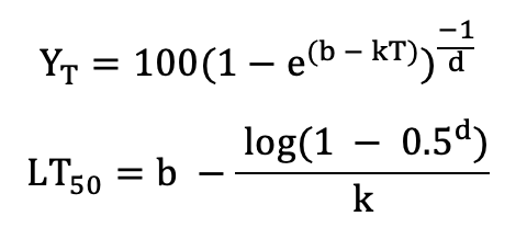
with YT the quantitative response variable at temperature T, and b, d, and k being function parameters;
Or the Gompertz function (Lim et al. 1998):
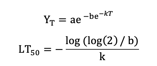
with the asymptote a, the x-placement parameter b and the slope-parameter k. Note that several other functions are in use, for example a symmetric function by Anderson et al. (1988):
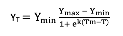
with Ymin the asymptotic value of the response variable in uninjured tissue, Ymax the asymptotic value at maximum low-temperature stress, k the steepness of the response curve, and Tm an estimate of LT50). Curve fitting can be carried out using non-linear least squares regression (a robust solution includes the nlsLM function in the minpack.lm R package; Elzhov et al. 2016). Note that many different equations can be used here, which is a drawback of this method in comparison to simple logistic regression of binary data.
Maintenance of freezing lab: this is dependent on conditions. If an ultra-low temperature lab is established (temperatures below −40 °C), costs for establishment and maintenance are much higher than for a lab at warmer temperatures, which can be achieved with commercial home freezers and a clever computer program. In any case, temperature in the samples should be measured independently and used in subsequent calculations of LT50 values.
Interpretation: survival of plants is a clear binary response, dead or alive. However, the obtained lethal temperature (LT50) is a statistical value, which does not imply that all individuals out of the studied population will die at this point. In addition, neither the entire organ nor the observed tissue may be dead, resulting in a gradual response for dead. How well LT50 values are related to survival of plants, which is the ultimate goal, is not known. Nevertheless, LT50 values of excised shoots and those measured in situ correlate strongly, although they are not the same (Neuner et al., 1997).
The usefulness of LT50, or the more general LD50, is the fact that one obtains a single value in units of the studied stress factor, which has ecological importance and can (at least within one study) be compared among species and organs. It should be noted, however, that this value depends not only on the dose, i.e. the minimum temperature, but also on duration of exposure, rate of cooling and warming, and the equation used. These facts therefore need to be reported alongside the results, but make a comparison among studies applying different protocols problematic.
5.4.2 Special cases, emerging issues, and challenges
Applying LD50 concepts to other stress factors in ecology beyond low temperature stress will not only advance stress ecology but, in the long run, also facilitate process-based projections of shifts in species composition with global change. Temporal dynamics in stress tolerance, however, need to be taken into account. Frost tolerance, for instance, does not only differ among species and populations, but also temporally over the course of the year (Lenz et al., 2013; Kreyling et al., 2015) and the phenological stage of a plant (Lenz et al., 2016b). In fact, frost tolerance responds dynamically to ambient temperatures within days (Kalberer et al., 2006; Lenz et al., 2016a; Vitra et al. 2017).
Concerning other stress factors, similar protocols as for frost tolerance can be applied. Drought tolerance, for instance, can be assessed by relative electrolyte leakage of plants or organs kept under osmotic stress which is caused experimentally by varying concentrations of polyethylene glycol in water solutions (PEG method; Premachandra & Shimada, 1987; Bajji et al., 2002).
Beyond the commonly reported LD50, other percentiles (e.g. LD10, LD90) can shed additional light on variation and range of stress tolerances.
Finally, it should be emphasised that accurate and correct measurements of the environmental variable studied is crucial. For instance, plant tissue temperature determines stress levels with regards to frost or heat. These tissue temperatures may deviate considerably from air temperatures. Using air temperatures might consequently lead to fairly nonsensical conclusions.
5.4.3 References
Theory, significance, and large datasets
Bigras et al. (2001), Chapter 4 in Snyder & de Melo-Abreu (2005), Sakai & Larcher (1987), Sakai & Weiser (1973), Thomashow (1999)
More on methods and existing protocols
Sakai & Larcher (1987) has a good chapter on protocols and how to measure freezing resistance. See also Hincha & Zuther (2014).
All references
Anderson, J. A., Kenna, M. P., & Taliaferro, C. M. (1988). Cold hardiness of Midiron and Tifgreen bermudagrass. Hortscience, 23(4), 748-750.
Bajji, M., Kinet, J.-M., & Lutts, S. (2002). The use of the electrolyte leakage method for assessing cell membrane stability as a water stress tolerance test in durum wheat. Plant Growth Regulation, 36(1), 61-70.
Bigras, F. J., Ryyppo, A., Lindstrom, A., & Sattin, E. (2001). Cold acclimation and deacclimation of shoots and roots of conifer seedlings. In F. J. Bigras, & S. J. Colombo (Eds.), Conifer Cold Hardiness (pp. 57-88). Dordrecht: Kluwer.
Bilavčík, A., Zámečník, J., Grospietsch, M., Faltus, M., & Jadrná, P. (2012). Dormancy development during cold hardening of in vitro cultured Malus domestica Borkh. plants in relation to their frost resistance and cryotolerance. Trees, 26(4), 1181-1192.
Buchner, O., & Neuner, G. (2009). A low-temperature freezing system to study the effects of temperatures to −70° C on trees in situ. Tree Physiology, 29(3), 313-320.
Ciais, P., Reichstein, M., Viovy, N., Granier, A., Ogee, J., Allard, V., … Valentini, R. (2005). Europe-wide reduction in primary productivity caused by the heat and drought in 2003. Nature, 437(7058), 529-533.
Clement, J. M. A. M., & van Hasselt, P. R. (1996). Chlorophyll fluorescence as a parameter for frost hardiness in winter wheat. A comparison with other hardiness parameters. Phyton-Annales Rei Botanicae, 36(1), 29-41.
Elzhov, T. V., Mullen, K. M., Spiess, A.-M., & Bolker, B. (2016). minpack.lm: R Interface to the Levenberg-Marquardt Nonlinear Least-Squares Algorithm Found in MINPACK, Plus Support for Bounds. https://CRAN.R-project.org/package=minpack.lm
Hincha, D. K. & Zuther, E. (Eds.) (2014). Plant Cold Acclimation. New York: Springer.
Kalberer, S. R., Wisniewski, M., & Arora, R. (2006). Deacclimation and reacclimation of cold-hardy plants: Current understanding and emerging concepts. Plant Science, 171, 3-16.
Kollas, C., Randin, C. F., Vitasse, Y., & Körner, C. (2014). How accurately can minimum temperatures at the cold limits of tree species be extrapolated from weather station data? Agricultural and Forest Meteorology, 184, 257-266.
Körner, C. (2012). Alpine Treelines, Functional Ecology of the Global High Elevation Tree Limits. Basel: Springer.
Kreyling, J., Persoh, D., Werner, S., Benzenberg, M., & Wöllecke, J. (2012). Short-term impacts of soil freeze-thaw cycles on roots and root-associated fungi of Holcus lanatus and Calluna vulgaris. Plant and Soil, 353(1-2), 19-31.
Kreyling, J., Schmid, S., & Aas, G. (2015). Cold tolerance of tree species is related to the climate of their native ranges. Journal of Biogeography, 42, 156-166.
Larcher, W. (2005). Climatic constraints drive the evolution of low temperature resistance in woody plants. Journal of Agricultural Meteorology, 61(4), 189-202.
Lenz, A., Hoch, G., Vitasse, Y., & Koerner, C. (2013). European deciduous trees exhibit similar safety margins against damage by spring freeze events along elevational gradients. New Phytologist, 200(4), 1166-1175.
Lenz, A., Hoch, G., & Vitasse, Y. (2016a). Fast acclimation of freezing resistance suggests no influence of winter minimum temperature on the range limit of European beech. Tree Physiology, 36(4), 490-501.
Lenz, A., Hoch, G., Körner, C., & Vitasse, Y. (2016b). Convergence of leaf‐out towards minimum risk of freezing damage in temperate trees. Functional Ecology, 30(9), 1480-1490.
Lim, C. C., Arora, R., & Townsend, E. C. (1998). Comparing Gompertz and Richards functions to estimate freezing injury in Rhododendron using electrolyte leakage. Journal of the American Society for Horticultural Science, 123(2), 246-252.
Lindén, L., Rita, H., & Suojala, T. (1996). Logit models for estimating lethal temperatures in apple. HortScience, 31(1), 91-93.
Munns, R., & Tester, M. (2008). Mechanisms of salinity tolerance. Annual Review of Plant Biology, 59, 651-681.
Neuner, G., & Hacker, J. (2012). Ice formation and propagation in alpine plants. In C. Lütz (Ed.), Plants in Alpine Regions (pp. 163-174). Vienna: Springer.
Neuner, G., Bannister, P., & Larcher, W. (1997). Ice formation and foliar frost resistance in attached and excised shoots from seedlings and adult trees of Nothofagus menziesii. New Zealand Journal of Botany, 35(2), 221-227.
Pramsohler, M., Hacker, J., & Neuner, G. (2012). Freezing pattern and frost killing temperature of apple (Malus domestica) wood under controlled conditions and in nature. Tree Physiology, 32(7), 819-828.
Premachandra, G. S., & Shimada, T. (1987). The measurement of cell membrane stability using polyethylene glycol as a drought tolerance test in wheat. Japanese Journal of Crop Science, 56(1), 92–98.
Räisänen, M., Repo, T., Rikala, R., & Lehto, T. (2006). Does ice crystal formation in buds explain growth disturbances in boron-deficient Norway spruce? Trees, 20(4), 441-448.
Sakai, A. (1960). Survival of the twig of woody plants at −196° C. Nature, 185(4710), 393-394.
Sakai, A. (1966). Studies of frost hardiness in woody plants. II. Effect of temperature on hardening. Plant Physiology, 41(2), 353-359.
Sakai, A., & Larcher, W. (1987). Frost Survival of Plants. Ecological Studies: Vol. 62. Berlin: Springer.
Sakai, A., & Weiser, C. J. (1973). Freezing resistance of trees in North America with reference to tree regions. Ecology, 54(1), 118-126.
Salazar-Gutiérrez, M. R., Chaves, B., & Hoogenboom, G. (2016). Freezing tolerance of apple flower buds. Scientia Horticulturae, 198, 344-351.
Siminovitch, D., Singh, J., & La Roche, I. A. D. (1978). Freezing behavior of free protoplasts of winter rye. Cryobiology, 15(2), 205-213.
Snyder, R. L, & de Melo-Abreu, J. P. (2005). Frost Protection: Fundamentals, Practice, and Economics. Rome: FAO
Steffen, K. L., Arora, R., & Palta, J. P. (1989). Relative sensitivity of photosynthesis and respiration to freeze-thaw stress in herbaceous species: Importance of realistic freeze-thaw protocols. Plant Physiology, 89(4), 1372-1379.
Sutinen, M. L., Palta, J. P., & Reich, P. B. (1992). Seasonal differences in freezing stress resistance of needles of Pinus nigra and Pinus resinosa – evaluation of the electrolyte leakage method. Tree Physiology, 11(3), 241-254.
Thomashow, M. F. (1999). Plant cold acclimation: Freezing tolerance genes and regulatory mechanisms. Annual Review of Plant Physiology and Plant Molecular Biology, 50, 571-599.
Trevan, J. W. (1927). The error of determination of toxicity. Proceedings of the Royal Society of London Series B: Biological Sciences, 101(712), 483-514.
Tylianakis, J. M., Didham, R. K., Bascompte, J., & Wardle, D. A. (2008). Global change and species interactions in terrestrial ecosystems. Ecology Letters, 11(12), 1351-1363.
Vitasse, Y., Lenz, A., Hoch, G., Körner, C., & Piper, F. (2014). Earlier leaf-out rather than difference in freezing resistance puts juvenile trees at greater risk of damage than adult trees. Journal of Ecology, 102(4), 981-988.
Vitra, A., Lenz, A., & Vitasse, Y. (2017). Frost hardening and dehardening potential in temperate trees from winter to budburst. New Phytologist, 216(1), 113-123.
Whitlow, T. H., Bassuk, N. L., Ranney, T. G., & Reichert, D. L. (1992). An improved method for using electrolyte leakage to assess membrane competence in plant tissues. Plant Physiology, 98, 198-205.
Authors: Kreyling J1, Lembrechts JJ2, De Boeck HJ2
Reviewer: Lenz A3
Affiliations
1 Experimental Plant Ecology, Institute of Botany and Landscape Ecology, University of Greifswald, Greifswald, Germany
2 Centre of Excellence PLECO (Plants and Ecosystems), Biology Department, University of Antwerp, Wilrijk, Belgium
3 Clinical Trial Unit Bern, Department of Clinical Research, University of Bern, Bern, Switzerland