Soils are physically composed of mineral and organic particles in varying sizes. The combined particles form the soil matrix that shapes the structure and pore spaces of soil. In turn, soil physical properties determine many key soil processes from soil water-holding capacity to cation exchange capacity that affect other life forms and ecosystem function. The key soil physical characteristics include soil structure, bulk density, and texture.
For the description of standard methods for soil characterisation we refer the reader to the Soil Science Society of America (SSSA) series on Methods of Soil Analysis; in particular, part 3 – Chemical Methods (Swift & Sparks, 2009) and part 4 – Physical Methods (Dane & Topp, 2002). Although the SSSA – Physical Methods (Dane & Topp, 2002) lists a complete set of methods, note that some of these traditional methods are being replaced by newer technology. In addition, the USDA Soil Survey Field and Laboratory Methods Manual (NRCS, 2014b) can be used as a new and simple guideline for methods in determining soil physical properties.
In this protocol, we focus on providing a basic guideline and starting point for determining soil physical properties in the context of climate-change studies as our main focus is on understanding ecosystem processes and plant behaviour.
Other variables that can be of relevance in some cases are described in Supporting Information S4. Water cycling (for example water potential and water repellency).
Soil samples
Several protocols in section 1.3 and 1.4 require sampling of soils. Here, we describe in general how to sample soil and important things that should be considered. Note that the sampling can vary considerably depending on the research question, method and individual needs (also check individual protocols for more details).
Before taking a soil sample the vegetation and litter (i.e. dead vegetation) are removed. Note that in some systems, litter can form a thick layer and be part of the organic horizon. Whether this layer is removed or not depends on the research question. The number of samples depends on many factors (e.g. research question, experimental design, finances, short-range variability in soil properties across the area of interest). A power analysis can give you a hint of the needed sample size. The soil is generally heterogenous and it is advisable to take a minimum of 3-5 soil samples per study unit (e.g. plot or block level). Samples from the same unit can also be pooled to represent the variability and reduce costs and time, but should be avoided if possible. Climate change experiments often have limited space for destructive sampling, and it is advisable to plan the soil sampling beforehand. If samples are taken from several plots with the same layout, it is advised to take samples in a fixed location within a plot and/or with similar aboveground vegetation. This helps the comparability between plots. The researcher should also consider if the variable of interest changes with time, which will determine if the sampling should be done once or several times.
For some measurements it can be necessary to use gloves and clean the equipment well between each soil sample to avoid contamination (e.g. genetic analysis).
The depth of the soil sampling depends on the method, research question and type of soil. It is advised to sample the whole soil profile (down to the bedrock) for pool size assessment, or at maximum root depth if the roots or microbial activity are the focus. Separate soil cores are usually taken from the organic layer defined as accumulated organic material on top of the mineral soil and mineral layer, but a higher resolution can be useful in deep soils and soils with several layers (Maaroufi et al., 2015).
Temporal scale (one time several times): if the aim is to assess total pool size of an element, it is advisable to sample only once as these numbers do not vary considerable with season. When the aim is to sample more dynamic pools (inorganic nutrients or microbial pool sizes) it is advisable to sample several times.
Spatial scale: if the aim is to assess the pool size in an area, it is recommended to take several soil samples, because the soil is often heterogeneous.
The size of the soil core depends a lot on the method, but often the diameter of the soil core is 3-8 cm. In general, structural and physical methods for measuring soil structure require diameters that are larger than the sampled soil depth to avoid damaging the soil structure. For processes related to microbial activity, it is advisable to take many small soil samples e.g. 10 samples with a 2 cm corer.
The amount of soil used is very variable and depends on the property of interest. For some methods it is crucial to know the volume of the soil sample (e.g. bulk density) to be able to scale up to an area basis, while for others a small amount of soil is needed (e.g. when concentrations or activity and not pool sizes are in focus).
Transport and storage – Each soil sample should be properly labelled including location, plot ID, profile number layer, depth, and date. The samples should not be exposed to the air or sun, as water will evaporate from the sample and warming can accelerate and activate unwanted biological processes. Soil samples are usually transported in plastic bags or boxes and kept cool during transport (ca. 4°C). For determination of very sensitive pools or processes, it may be recommended to place samples in a cooler with dry ice (e.g. for extraction of soil enzymes). Ideally, the soil is analysed immediately after sampling, and some methods require quicker processing than others. Often quick processing is however not possible (e.g. due to continuous field work) and then the soils should be stored in the proper way. There is no general rule for how to store soil before the analysis and it depends on the origin of the soil and the purpose and method. For example, tropical soils should not be stored in a fridge, since the low temperature can kill microbes and soil lysis will lead to underestimation of the microbial biomass. However if soil is sampled frozen in cold environments (e.g. arctic), then the samples should be kept frozen until the analysis. For some methods and soils the fridge or freezer is recommended for storage, while for others air or oven drying is the best practice.
For some analyses, the roots and stones (>2 mm) are removed from the soil samples, using a sieve of 2 mm mesh width. If the total mass of the samples needs to be known, the removed parts are weighed (e.g. for bulk density). This is especially important for stony soils. For measurements that require undisturbed soil (e.g. many physical measurements), the stones are not removed.
The soil samples are often used fresh, but for some analysis the soil needs to be dried. However, this depends largely on what the samples are used for. Soils can be dried at room temperature, low oven temperature or higher temperature. Table 1.3.1 shows how to process soil samples for the most commonly used methods (for more details check individual protocols).
Table 1.3.1 Temperature for processing soil samples for common methods.
| Temperature for drying | Method | Protocol |
| Fresh soil kept in fridge (4°C)
|
Soil microbial biomass
Soil enzymatic activity PLFA Soil activity assays Bulk density pH |
2.2.1
1.3.4 1.4.1 |
| Air dried, room temperature (25°C) | Soil water repellency | 3.6 |
| Oven dried, low temperature (max. 55°C) | Soil carbon and nutrient stocks | 2.2.4 |
| Oven dried, high temperature (70° – 105°C) | SOM (loss on ignition) | 1.4.2 |
Where to start
The International Co-operative Programme on Assessment and Monitoring of Air Pollution Effects on Forests (Cools & De Vos, 2016) and the Countryside Survey (Emmett et al., 2010) give a good overview over how to sample soils.
1.3.1 Soil types and horizons (layers)
Unlike sediments that are deposited over time, soils are developed as horizons from the parent material under the influence of local climate, topography, and biota. There are many soil types based on the composition of the parent material, texture, and organic matter. A soil horizon is a parallel layer to the soil surface with distinctly different physical, chemical, and biological characteristics from the layers above or beneath. A vertical layout of a soil (based on a soil pit) illustrates the different horizons in a soil profile (Figure 1.3.1). Determining soil horizons within a soil profile will provide important information about the life history of the soil as well as different characteristics of soil properties.
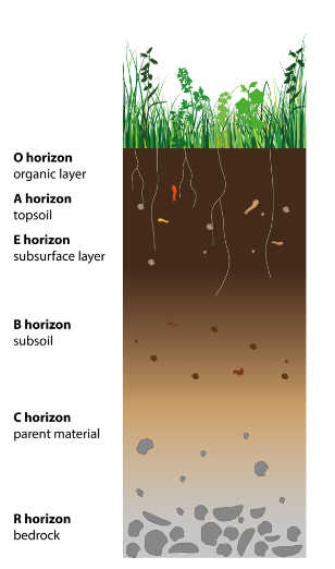
The soil profile should be described according to a soil classification that is compatible with the World Reference Base (WRB) system. Soil type should be reported according to the World Reference Base for Soil Resources system (ISRIC, 1998; IUSS Working Group WRB, 2006, 2014). This is the international standard taxonomic soil classification system, which is endorsed by the International Union of Soil Sciences (IUSS) and replaces the FAO soil classification. Reporting the depth of soil layers or horizons should be included in any description as this is important for comparison and modelling. Most classification systems recognise six master soil horizons which are designated using the capital letters O, A, E, B, C, and R (Figure 1.3.1). Reporting O to B is usually sufficient for climate-change studies. O = Organic matter, characterised by high levels of organic material: dark in colour; A = Mineral topsoil, often organically stained: contains highly weathered parent material (rocks) and is lighter in colour than the O horizon; E = Eluviated – used to label a horizon that has been highly leached of minerals, clays, and sesquioxides: usually determined as a pale layer below the A horizon and only exists in older, well-developed soils; B = Subsoil, an illuviated layer that accumulates iron, clay, aluminium, and organic compounds: lighter in colour and often may be reddish due to the iron content; C = Broken-down bedrock, also known as substratum; R = Bedrock.
What and how to measure?
Traditionally, determining soil horizons involves excavating a pit exposing a clean vertical surface of approximately 1 metre depth and identifying the depths of different horizons based on colour and physical properties. This can be simplified by using a soil auger. First, identify the depth of soil until the bedrock or parent material layer. Using a soil auger, sample the continuous soil profile until bedrock or parent material is reached, and identify horizons based on different characteristics. Samples are often collected and taken back to the laboratory for analysis. A wide number of texts are available that describe soil analysis: those more widely used include NRCS (2014a) and Dane & Topp (2002).
1.3.2 Plant rooting depth and distribution by depth
The plant rooting depth is important to measure the distribution of roots throughout the soil profile as this may change when the plants are subjected to climatic treatments. If the site is heterogeneous (e.g. slope or changes in vegetation), rooting depth should be determined in more than one place. Plant rooting depth is measured by digging a soil profile (see 1.3.1 Soil horizon) and can be measured when the soil layers are determined.
1.3.3 Stone content (%)
Stone content defines the volume and mass in the soil containing stones > 2 mm. Stones do not contribute to plant nutrient supply or water-holding capacity in the soil and the weight and volume of stones are most often subtracted when > 5% of the soil volume (ICP, 2016). To calculate the stone content, an air-dried soil sample of known mass is sieved so that stones larger than 2 mm are removed. The stones are weighed and the % of stones above 2 mm can be determined and reported as a % of the total mass of soil.
1.3.4 Bulk density (g cm–³)
Bulk density is a measure of the amount of soil per unit volume of oven dried soil and gives information on the physical status of the soil. The soil organic matter content, soil texture, the minerals in the soil and degree of compaction define the bulk density. Bulk density varies substantially among soils. Mineral soils have a bulk density of around 1–1.6 g cm–³, while in organic soils and friable clay it is well below 1 g cm–³. Bulk density values are essential when determining soil carbon and nutrient stocks, as they allow a conversion from concentrations to mass per area (see also protocol 2.2.4 Soil carbon and nutrient stocks).
What and how to measure?
A range of equipment is available for the determination of bulk density and general guidance can be found in Grossman & Reinsch (2002). A volumetric core (the volume must be known), which should be at least 75 mm in diameter, with the depth no greater than the diameter, should be taken down the soil profile, ideally at 5 cm increments. Although dry bulk density can be determined on the entire soil sample (with stones), it is usually reported for soil sieved through 2 mm mesh, the fine-earth fraction, which is suitable for subsequent calculations of carbon and nutrient stocks. The stones (> 2mm) are removed and weighed separately. The soil samples are dried at 105°C and then weighed.
Dry bulk density is calculated using the following equation:

The stone volume can be determined through the water displacement method using this equation:
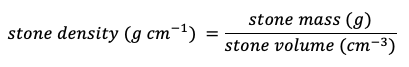
The stone density is usually assumed to be ~2.65 g cm–³.
Resampling of bulk density is normally not required. However, especially severe drought may change the bulk density and resampling of bulk density is recommended after 3–5 years.
1.3.5 Soil texture
Soil texture is the particle size distribution of soil determined by a percent combination of sand, silt, and clay that presents coarseness of a soil. Soil texture partly determines soil water-holding capacity and permeability, which provides important characteristic information about soil physical properties. The percentage clay in particular is also highly relevant for nutrient availability, as the clay colloids serve as exchange places for cations such as NH4+, K+, Ca2+ and Mg2+, similarly to humus particles.
What and how to measure?
Particle size analysis (PSA) is used in soil science to determine soil texture (sand, silt, and clay content), and often used in soil physics to determine soil hydraulic properties. PSA is often reported for the fine earth fraction of soils < 2 mm in diameter. Soil samples returning to the laboratory are usually sieved to remove particles > 2mm and root material. PSA can be determined using sedimentation with either the pipette method or the hydrometer method (Gee & Or, 2002). The texture of soil is expressed using the soil textural triangle from the composition of different particles (NRCS, 2014b). Texture in organic soils is not measured.
1.3.6 Water table depth (m)
The water table is the upper extent of the phreatic or groundwater zone, in which all soil pores and fractures are completely filled with water. The water table marks the end of the vadose zone. The phreatic zone and therefore the water table depth may vary between seasons and with dry or wet periods.
In areas with shallow water tables, for example in deltaic areas (van der Ploeg et al., 2012) or wetlands (Oosterwoud et al., 2017), or in soils with a perched water table owing to less permeable soil layers, the water table influences the amount of water available for vegetation and soil evaporation. For vegetation, the water table influences water availability as roots may grow towards the water table or via capillary rise of groundwater. Capillary rise is a physical phenomenon where water will rise in a hollow tube with a small diameter. The smaller the tube the higher the water will rise. Soil pores form a network of such hollow tubes, and the height of capillary rise depends on the soil texture and structure (Brutsaert, 2005, section 9.6), leading to a range from 0.2–0.5 m capillary rise for coarse textured soil (e.g. sand) to 0.8–several m for fine textured soil (e.g. clay). For soil evaporation, water is transported from the underlying soil layers by liquid and vapour transport, which can be influenced by groundwater through capillary rise. If the water table is expected to influence the climate-change studies it is recommended to monitor the water table fluctuations.
What and how to measure
The water table can be measured with a piezometer, which is a tube with a perforated, screened part for groundwater to enter the tube while soil material is kept out (Reeve, 1986). It can be installed by drilling a hole manually with a soil auger or with drilling equipment. Before installing in a site with perched water tables, ensure that the site’s less permeable layers are not drained by making holes through them, thus altering the soil hydraulics. Once the piezometer is installed, measurements can be done manually with a measurement tape with a float or automatically with a pressure transducer (e.g. Oosterwoud et al., 2017).
1.3.7 References
Brutsaert, W. (2005). Hydrology: An Introduction. Cambridge: Cambridge University Press.
Dane, J. H., & Topp, G. C. (Eds.). (2002). Methods of soil analysis: Part 4—Physical methods. In J. H. Dane, & C. G. Topp (Eds.), Methods of Soil Analysis (pp. 1018–1020). Madison, WI: Soil Science Society of America, American Society of Agronomy.
Gee, G. W., & Or, D. (2002). 2.4 Particle-size analysis. In J. H. Dane, & C. G. Topp (Eds.), Methods of Soil Analysis: Part 4—Physical Methods (pp. 255–293). Madison, WI: Soil Science Society of America.
Grossman, R. B., & Reinsch, T. G. (2002). 2.1 Bulk density and linear extensibility. In J. H. Dane, & C. G. Topp (Eds.), Methods of Soil Analysis: Part 4—Physical Methods (pp. 201–228). Madison, WI: Soil Science Society of America.
ISRIC International Soil Reference and Information Centre. (1998). World Reference Base for Soil Resources. World Soil Resources Reports 84. Rome, FAO.
IUSS Working Group WRB. (2006). World Reference Base for Soil Resources 2006: A Framework for International Classification, Correlation and Communication. Rome, FAO.
IUSS Working Group WRB. (2014). World Reference Base for Soil Resources 2014: International Soil Classification System for Naming Soils and Creating Legends for Soil Maps (3rd ed.). Rome, FAO.
Maaroufi, N. I., Nordin, A., Hasselquist, N. J., Bach, L. H., Palmqvist, K., & Gundale, M. J. (2015). Anthropogenic nitrogen deposition enhances carbon sequestration in boreal soils. Global Change Biology, 21(8), 3169-3180.
NRCS Natural Resources Conservation Service. (2014a). Soil Electrical Conductivity: Soil Health – Guides for educators. United States Department of Agriculture.
NRCS Natural Resources Conservation Service. (2014b). Soil Survey Field and Laboratory Methods Manual, Soil Survey Investigations Report No. 51 (Version 2.0.). United States Department of Agriculture.
Oosterwoud, M., van der Ploeg, M., van der Schaaf, S., & van der Zee, S. (2017). Variation in hydrologic connectivity as a result of microtopography explained by discharge to catchment size relationship. Hydrological Processes, 31(15), 2683–2699.
Reeve, R. C. (1986). Water potential: piezometry. In A. Klute (Ed.), Methods of Soil Analysis: Part 1—Physical and Mineralogical Methods (pp. 545–561). Madison, WI: Soil Science Society of America, American Society of Agronomy.
Swift, R. S., & Sparks, D. L. (2009). Methods of Soil Analysis: Part 3—Chemical Methods. In D. L. Sparks, A. L. Page, P. A. Helmke, & R. H. Loeppert (Eds.), Soil Science Society of America Book Series, 5. Madison, WI: Soil Science Society of America, American Society of Agronomy.
Van der Ploeg, M. J., Appels, W. M., Cirkel, D. G., Oosterwoud, M. R., Witte, J.-P. M., & van der Zee, S. E. A. T. M. (2012). Microtopography as a driving mechanism for ecohydrological processes in shallow groundwater systems. Vadose Zone Journal, 11, 3.