Weather includes abiotic factors that impact the functioning of an ecosystem. Meteorological databases can provide fundamental information for climatological and climate-change studies. These observations can be taken manually (weather observer), in automated mode (data-logging system applications or weather station data), or in a hybrid scheme where weather observer efforts are supplemented by automated weather measurements. The most commonly measured meteorological parameters relevant to studies of land–plant–atmosphere interactions are those relating to energy and water fluxes (De Boeck et al., 2017), which in turn affect ecosystem carbon dynamics. Precipitation inputs (e.g. rain and/or snow) and rates of evapotranspiration (commonly estimated on the basis of air temperature, relative humidity, and wind speed values) are needed for water budget assessments. The meteorological systems, both manual and automated, require permanent supervision due to the complex and often harsh ambient conditions. The World Meteorological Organization (WMO) has prepared an extensive reference work on meteorological observations that can be found online (WMO, 2012).
1.5.1 Weather station and nearby weather station data
A climate-change studies should be equipped with a weather station for measuring climate drivers. A wide variety of weather stations are available but a high quality and reliable automated weather station (hereafter AWS) that is calibrated is desirable. An AWS consists of a weather-proof enclosure containing data logger, telemeter (optional), and meteorological sensors. The whole system should be mounted on a mast and it is powered and backed-up with a battery that is charged with a solar panel, wind turbine, or regular power line if available. The weather station should be mounted above the studied plant canopy. Microclimate often varies considerably across the ground-atmosphere interface (Graae et al., 2012). If possible, multiple measurements should be taken, and in such a manner as to make them relevant for the biotic question at hand (for example, within the soil, on the surface, and/or in the vegetation canopy, inside/outside experimental structures such as open-top chambers (OTC) or rainout shelters) while at the same time allowing calibration with climate station data (which are typically taken 2 m above ground). The specific configuration may vary based on the purpose of the system and local conditions, thus the measurements must be defined before the study. Meteorological measurements that are influenced by an experimental treatment (e.g. air and soil temperature, soil moisture in OTC) should be repeated at each experimental treatment preferably with replicates, and variables that vary across the site should preferably be measured at the block or plot scale (Lamentowicz et al., 2016). These plot-level temperature and rainfall measurements, combined with the site-level AWS data, provide the minimum data needed to monitor and assess whether the planned experimental modifications of climate drivers are being achieved. For all the instruments we recommend using the manufacturer’s instructions regarding set-up and use.
The system may report in real-time using telemetry, which is generally more energy demanding, or record data for collection later. The real-time measurements allow early detection of measuring process disruption, for example logger or sensor failure, and hence might minimise climate data loss, whereas a non-telemetric scheme of the system operation requires visits to the site providing opportunities to inspect the study and enable eventual repairs of the system. Whether to use telemetry or not might be determined by the accessibility of the site, the type of power source, and additional routine manual observation requirements.
Separate sensors connected to the AWS can monitor air temperature, relative humidity, barometric pressure and tendency (change in pressure), wind speed and direction, total, net and photosynthetically active shortwave and longwave radiation fluxes, rainfall and water equivalent snowfall, and snow depth (if relevant). Additionally, soil moisture, soil temperature, and soil matric potential may be observed. Many of the soil moisture sensors measure temperature alongside. This reduces the number of applied sensors and consequent soil disruption. The installation of sensors will depend on the type and configuration of the instrument, but some general approaches to installation can be identified.
New technological advancement coming up with small climate stations that can be placed inside the plots of most climate change experiments and measure multiple microclimate variables for long time periods. One newly developed mini climate station is the tomst TMS-4 data logger, that measures air and soil temperature and soil moisture and has proved to produce reliable data for a range of different habitats (Wild et al., 2019).
Soil sensors are often used to monitor seasonal changes of the soil environment parameters. Daily changes occur, but can often be considered noise against the slower seasonal signal. Rather than measuring at fixed depths, it is of interest to know the moisture and temperature – and matric potential if measured – near the soil surface, e.g. within 5–15 cm. In shallow soils such as in alpine areas, 3–5 cm is recommended (Körner & Hiltbrunner, 2018) at a point corresponding to the maximum root density (Figure 1.5.1). In the best of all worlds, a second set of sensors would be placed at greater depth, perhaps near the bottom of the root system. Such positioning would capture the rare drought or snowmelt events that deplete or refill the whole soil profile moisture. In boreal forests, these deeper sensors are often placed at 50 cm below the surface. As much as we would like to standardise these depths, the variation in diurnal/seasonal cycles and in root water depletion depths prevents convergence on a single recommendation.
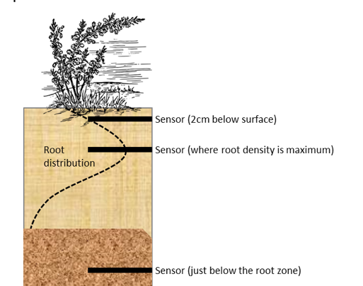
When installing sensors in a plot it is generally best to install them horizontally (to measure temperature at the desired depth), which can be achieved by excavating a small trench from outside the plot into the plot (Figure 1.5.1). This prevents preferential flow of water along the cables.
Generally, in areas with rodents, it can be useful to protect the wire of a sensor with PVC tubes to prevent damage. In alpine areas, where there is a lot of snow in spring, it can be advisable to protect the wire higher up, because rodents can climb up on the snow.
For each of the sensors, the optimal sampling interval is every minute and should be reported in the form of half-hourly to hourly averages. For example, modelling of ecosystem gas exchange will require half-hourly (e.g. Papale et al., 2006) to hourly data input.
Data management: high-resolution AWS data need to be quality checked due to the possibility of malfunctioning sensors, lack of power supply or system failures etc. The automated quality control procedures are used for selection (flagging) of uncertain data and the final data quality assessment must be performed by professional personnel that are familiar with local conditions. This visual inspection can be done with basic graphic tools that plot the data and trends for all measurements. Although this method seems less accurate than setting prescribed limits that data must fit within, it does allow for human interpretation and recall of conditions at the site – for example, an automated limit in a script will fail to remember if it was a particularly cold week.
Reporting climate data: when reporting climate data it is important to specify the timeframe in which the data were collected, name of the location if the data were obtained from a weather station, and (if applicable) explain any data processing (e.g. summer temperature, daily mean, cumulative temperature; Morueta-Holme et al., 2018).
Meteorological measurements
A site-based AWS should measure air, soil, and canopy temperature, relative humidity, photosynthetic photon flux density (PPFD), soil moisture, rainfall, and, in windy regions, wind speed (and, if relevant, direction). These measurements will help put plot-level data into context as, for example, air temperature and photosynthetically active radiation affect the level of photosynthetic uptake of atmospheric CO2 by plants. They are also necessary for gap-filling eddy covariance gas flux measurements (protocol 2.3.1 Ecosystem CO2 and trace gas fluxes), used to quantify the greenhouse gas balance of multiple ecosystem types (Kang et al., 2018).
1.5.2 Air temperature (°C)
Among other variables, air temperature affects tissue, canopy, and soil temperature and is thus relevant for plant growth, water cycling, microbial activity, and phenological response, and therefore the level of photosynthetic uptake of atmospheric CO2 by plants.
Air temperature should be measured at 2 m above the ground surface, as this is a standard height to compare with weather station data; however, measuring air temperature in the canopy and at ground level is biologically more relevant for the plants. Standard heights for measuring canopy temperature are 20 cm and ground level in low vegetation, and above the canopy in high vegetation, such as forests (Barr et al., 2007; Reichstein et al., 2007). For experiments that affect temperature it is important to measure the treatment effects. For example, an OTC will not affect the air temperature at 2 m.
Tissue temperature, which is relevant for metabolic rates and the water cycle, can be measured directly using infrared thermometers (protocol 5.5 Leaf temperature).
Air temperature should be measured every 1–10 minutes, from which daily minimum, maximum, and cumulative temperature sum can be calculated. The daily minimum and maximum air temperature can be used for a rough estimate of potential evapotranspiration using the Hargreaves equation (Jensen et al., 1997).
1.5.3 Soil temperature (°C)
Soil temperature is a primary driver of biogeochemical reactions, impacting responses that climate-change studies often quantify, such as soil respiration (carbon efflux) and nitrogen mineralisation (Knoepp & Swank, 2002; Curtis et al., 2005, also see protocol 3.5 Soil temperature).
Sensors should be installed horizontally and installation depths vary depending on the study objective. When associated with soil respiration or decomposition, sensors should, at minimum, be installed 5 cm beneath the soil surface (Wangdi et al., 2017). For leaf litter decomposition, an additional sensor should be placed at a depth of 2 cm. Soil microbial studies may require temperature profiles layered deeper in the soil (Angle et al., 2017; Che et al., 2018). At least one sensor at each depth should be installed in every plot, more in environmentally heterogeneous plots, such as those with varying topography. Sensors should be connected to a data logger and take measurements every 1–15 minutes. In the absence of a meteorological tower, for example when portable chamber-based gas flux measurements are applied, soil temperature can be measured with handheld thermometer probes or thermocouples installed within the chamber (Collier et al., 2014).
SOILTEMP is an initiative to build a global soil temperature database to provide more relevant temperature data for species.
1.5.4 Photosynthetic photon flux density PPFD (μmol m-2 s-1)
Photosynthetically active radiation (PAR) is defined as the spectral range of solar radiation (0.4–0.7 μm) that is used by plants within the process of photosynthesis. The density of the flux of these light molecules is called photosynthetic photon flux density (PPFD) and is a quantitative measure of the energy that reaches the plant canopy. PPFD impacts the rate at which plants photosynthesise, affecting growth and carbon storage. PPFD data are used to calculate scattered light conditions (cloudiness), sunshine hours, and light-use efficiency (LUE), as well as in gap-filling eddy covariance gas flux measurements. In forest ecosystems, multiple sensors can be used to partition LUE of the canopy and sub-canopy, which is important when determining the recovery response (Reed et al., 2014; Stuart-Haëntjens et al., 2015).
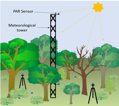
One sensor should be mounted above the vegetation, on top of the meteorological platform or tower, positioned to avoid shading by other instrumentation. Due to cloud variation, PPFD should not be retrieved from nearby weather stations. Light environments below a forest canopy will likely change following climate manipulation experiments, so when a sub-canopy is present, additional sensors should be placed between the sub-canopy and canopy, and on the ground surface (Figure 1.5.2). Multiple sensors installed below the canopy capture the heterogeneous light conditions. Sensors installed between the canopy and sub-canopy can be mounted and levelled lower on the meteorological tower, on small tripods, or on hand-made PVC poles.
1.5.5 Relative humidity (%)
Relative humidity in combination with air temperature is used to calculate vapour pressure deficit, which can impact plant mortality, stomatal conductance, and, consequently, greenhouse gas fluxes (Breshears et al., 2009; Will et al., 2013; Yuan et al., 2016). This metric is growing more important as temperature increases due to climate change also raise atmospheric moisture demand, unless relative humidity increases (Breshears et al., 2013).
Relative humidity sensors can be installed on a meteorological station or tower, and in forests, should be placed above the canopy as well as below the canopy to assess sub-canopy growth dynamics.
1.5.6 Precipitation (mm)
Precipitation is often measured in climate-change studies, because it indicates the amount of water entering a system. It should, however, be stressed that precipitation is not the amount of water available for plants. Depending on the soil and prior meteorological conditions (e.g. a drought period), a considerable amount is intercepted by plant canopy, runs off, or drains into deeper layers of the soil. As such, soil moisture is a better measure of water availability for plants.
A ground-level storage rain gauge collects rain accumulated over a given period of time. Accumulated rainfall is measured in mL of water and converted to mm or rain where Rain [mm] = Rain [mL] / πr2Funnel [m2] of the rain gauge. The quantity of rainfall accumulated should never exceed the storage capacity of the gauge. Therefore, the frequency of emptying the rain gauge depends on the precipitation in a given area. Data from ground-level rain gauges are robust and far less vulnerable to issues such as logger downtime or loss of power, etc. In tall vegetation (e.g. forest), readings are often biased by turbulence, and usually precipitation data must be adopted from a nearby location.
The tipping bucket rain gauge consists of a plastic collector that is balanced over a pivot and collects the precipitation. A pre-set amount of precipitation tips the collector and actuates a switch which is then electronically recorded or transmitted to a remote collection station. The tipping bucket can be less accurate, i.e. if the rain stops before the lever has tipped, which is then added to the next rainfall event. Also, heavy rainfall and snow events are often underestimated with tipping buckets (WMO, 2012). In places with high vegetation, falling leaves and needles can plug the rain gauge and should therefore often be checked and cleaned.
Plot treatments such as drought or any rain-interfering structures such as scaffolding, will alter the plot-level rainfall input, therefore measuring direct water inputs to the plots is important. Often a simple manual rain gauge is sufficient on treatment plots.
1.5.7 Soil moisture
Soil moisture is the amount of water in the soil (Robinson et al., 2008; Vereecken et al., 2008). It provides the biological moisture pool for microbial activity and plant transpiration supporting terrestrial life. Soil moisture dynamics are likely to respond in different ways to climate change, depending on whether it leads to drought, warming, or excess rainfall (Seneviratne et al., 2010). This will have a direct effect on the biologically available moisture pool, and oxygen levels in the case of wet soils. Moreover, because soil moisture controls microbial activity, carbon and nutrient cycling will be affected, as will greenhouse gas fluxes such as CO2, CH4, and N2O.
For how to measure soil moisture see protocol 3.1 Soil moisture.
1.5.8 Rain throughfall
In manipulation experiments where the experimental structures may reduce the amount of rainwater that enters the experimental plots, rain throughfall may be measured. Throughfall is measured easiest with a funnel-storage bottle construction which is placed into the plant canopy. The volume of throughfall is measured at the same time as rainfall accumulated by the rain gauge. In cold regions, bottles need to be exchanged and then thawed in the laboratory for the rain volume to be recorded. The rain throughfall volume on a plot basis is then converted to mm rainfall using the funnel diameter (see 1.5.6 Precipitation). Throughfall and rain gauge values are used to calculate a percentage reduction in rainfall per plot.
1.5.9 Wind speed (m s-1) and direction (degrees)
Wind speed and direction can help to interpret temperature measurements, snowmelt date and photosynthetic activity, and is most often associated with ecosystem scale gas flux measurements obtained by eddy-covariance flux towers. Sonic anemometers should be installed at 1.5–2 times vegetation height. Calculations of wind speed and direction may need to be adjusted in hilly terrain (Zitouna-Chebbi et al., 2015).
1.5.10 References
Angle, J. C., Morin, T. H., Solden, L. M., Narrowe, A. B., Smith, G. J., Borton, M. A., … Wrighton, K. C. (2017). Methanogenesis in oxygenated soils is a substantial fraction of wetland methane emissions. Nature Communications, 8(1), 1567.
Barr, A. G., Black, T. A., Hogg, E. H., Griffis, T. J., Morgenstern, K., Kljun, N., … Nesic, Z. (2007). Climatic controls on the carbon and water balances of a boreal aspen forest, 1994–2003. Global Change Biology, 13(3), 561–576.
Breshears, D. D., Myers, O. B., & Meyer, C. W. (2009). Tree die‐off in response to global change‐type drought: Mortality insights from a decade of plant water potential measurements. Frontiers in Ecology and the Environment, 7(4), 185–189.
Breshears, D. D., Adams, H. D., Eamus, D., McDowell, N. G., Law, D. J., Will, R. E., … Zou, C. B. (2013). The critical amplifying role of increasing atmospheric moisture demand on tree mortality and associated regional die-off. Frontiers in Plant Science, 4, 266.
Che, R., Deng, Y., Wang, W., Rui, Y., Zhang, J., Tahmasbian, I., … Cui, X. (2018). Long-term warming rather than grazing significantly changed total and active soil procaryotic community structures. Geoderma, 316, 1–10.
Collier, S. M., Ruark, M. D., Oates, L. G., Jokela, W. E., & Dell, C. J. (2014). Measurement of greenhouse gas flux from agricultural soils using static chambers. Journal of Visualized Experiments, 90, e52110.
Curtis, P. S., Vogel, C. S., Gough, C. M., Schmid, H. P., Su, H.-B., & Bovard, B. D. (2005). Respiratory carbon losses and the carbon-use efficiency of a northern hardwood forest, 1999–2003. New Phytologist, 167(2), 437–456.
De Boeck, H. J., Kockelbergh, F., & Nijs, I. (2017). More realistic warming by including plant feedbacks: A new field-tested control method for infrared heating. Agricultural and Forest Meteorology, 237-238, 355–361.
Graae, B. J., De Frenne, P., Kolb, A., Brunet, J., Chabrerie, O., Verheyen, K., … Milbau, A. (2012). On the use of weather data in ecological studies along altitudinal and latitudinal gradients. Oikos, 121(1), 3–19.
Jensen, D. T., Hargreaves, G. H., Temesgen, B., & Allen, R. G. (1997). Computation of ETo under non-ideal conditions. Journal of Irrigation and Drainage Engineering, 123(5), 394–400.
Kang, M., Kim, J., Thakuri, B. M., Chun, J., & Cho, C. (2018). New gap-filling and partitioning technique for H2O eddy fluxes measured over forests. Biogeosciences, 15(2), 631–647.
Knoepp, J. D., & Swank, W. T. (2002). Using soil temperature and moisture to predict forest soil nitrogen mineralization. Biology and Fertility of Soils, 36(3), 177–182.
Körner, C., & Hiltbrunner, E. (2018). The 90 ways to describe plant temperature. Perspectives in Plant Ecology, Evolution and Systematics, 30, 16–21.
Lamentowicz, M., Słowińska, S., Słowiński, M., Jassey, V., Chojnicki, B. H., Reczuga, M. K., … Buttler, A. (2016). Combining short-term manipulative experiments with long-term palaeoecological investigations at high resolution to assess the response of Sphagnum peatlands to drought, fire and warming. Mires and Peat, 18(20), 1–17.
Morueta-Holme, N., Oldfather, M. F., Olliff-Yang, R. L., Weitz, A. P., Levine, C. R., Kling, M. M., … Ackerly, D. D. (2018). Best practices for reporting climate data in ecology. Nature Climate Change, 8(2), 92–94.
Papale, D., Reichstein, M., Aubinet, M., Canfora, E., Bernhofer, C., Kutsch, W., … Yakir, D. (2006). Towards a standardized processing of Net Ecosystem Exchange measured with eddy covariance technique: algorithms and uncertainty estimation. Biogeosciences, 3(4), 571–583.
Reed, D. E., Ewers, B. E., & Pendall, E. (2014). Impact of mountain pine beetle induced mortality on forest carbon and water fluxes. Environmental Research Letters, 9(10), 105004.
Reichstein, M., Ciais, P., Papale, D., Valentini, R., Running, S., Viovy, N., … Zhao, M. (2007). Reduction of ecosystem productivity and respiration during the European summer 2003 climate anomaly: a joint flux tower, remote sensing and modelling analysis. Global Change Biology, 13(3), 634–651.
Robinson, D. A., Campbell, C. S., Hopmans, J. W., Hornbuckle, B. K., Jones, S. B., Knight, R., … Wendroth, O. (2008). Soil moisture measurement for ecological and hydrological watershed-scale observatories: A review. Vadose Zone Journal, 7(1), 358–389.
Seneviratne, S. I., Corti, T., Davin, E. L., Hirschi, M., Jaeger, E. B., Lehner, I., … Teuling, A. J. (2010). Investigating soil moisture–climate interactions in a changing climate: A review. Earth-Science Reviews, 99(3), 125–161.
Stuart-Haëntjens, E. J., Curtis, P. S., Fahey, R. T., Vogel, C. S., & Gough, C. M. (2015). Net primary production of a temperate deciduous forest exhibits a threshold response to increasing disturbance severity. Ecology, 96(9), 2478–2487.
Vereecken, H., Huisman, J. A., Bogena, H., Vanderborght, J., Vrugt, J. A., & Hopmans, J. W. (2008). On the value of soil moisture measurements in vadose zone hydrology: A review. Water Resources Research, 44(4), WOOD06.
Wangdi, N., Mayer, M., Nirola, M. P., Zangmo, N., Orong, K., Ahmed, I. U., … Schindlbacher, A. (2017). Soil CO2 efflux from two mountain forests in the eastern Himalayas, Bhutan: components and controls. Biogeosciences, 14(1), 99–110.
Wild, J., Kopecký, M., Macek, M., Šanda, M., Jankovec, J., & Haase, T. (2019). Climate at ecologically relevant scales: A new temperature and soil moisture logger for long-term microclimate measurement. Agricultural and forest meteorology, 268, 40-47.
Will, R. E., Wilson, S. M., Zou, C. B., & Hennessey, T. C. (2013). Increased vapor pressure deficit due to higher temperature leads to greater transpiration and faster mortality during drought for tree seedlings common to the forest-grassland ecotone. New Phytologist, 200(2), 366–374.
WMO. (2012). Guide to Meteorological Instruments and Methods of Observation. WMO-No. 8. 2008 edition updated 2010. World Meteorological Organization.
Yuan, W., Cai, W., Chen, Y., Liu, S., Dong, W., Zhang, H., … Zhou, G. (2016). Severe summer heatwave and drought strongly reduced carbon uptake in Southern China. Scientific Reports, 6, 18813.
Zitouna-Chebbi, R., Prévot, L., Jacob, F., & Voltz, M. (2015). Accounting for vegetation height and wind direction to correct eddy covariance measurements of energy fluxes over hilly crop fields. Journal of Geophysical Research, D: Atmospheres, 120(10), 4920–4936.